Sparse Autoencoder Universality - Under What Conditions are Learned Features Consistent?

This project aims to study the universality of features in LLMs by studying sparse autoencoders trained on similar layers of different models.

Introduction

Neural networks are black boxes. We understand the process by which they are created, but just as understanding the principle of evolution yields little insight into the human brain, designing a model’s optimization process yields little insight into how that model reasons. The field of mechanistic interpretability attempts to understand how human-understandable concepts combine within a model to form its output. With sufficiently good interpretability tools, we could ensure reasoning transparency and easily find and remove harmful capabilities within models (such as hallucinations) .

In 2022, Anthropic identified a core challenge in interpreting a model’s reasoning layer-by-layer: polysemanticity, a phenomenon in which a single neuron activates for many different concepts (e.g. academic citations, English dialogue, HTTP requests, and Korean text). This is a result of a high-dimensional space of concepts (‘features’) being compressed into the lower-dimension space of the neural network . Sparse autoencoders, a form of dictionary learning, help to linearly disentangle polysemantic neurons into interpretable features .

Sparse autoencoders work by projecting a single layer of a neural network into a higher-dimension space (in our experiments, we train autoencoders ranging from a 1:1 projection to a 1:32 projection) and then back down to the size of the original layer. They are trained on a combination of reconstruction loss, their ability to reconstruct the original input layer, and a sparsity penalty, encouraging as many weights as possible to be 0 while retaining good performance

Setup

(https://www.alignmentforum.org/posts/wqRqb7h6ZC48iDgfK/tentatively-found-600-monosemantic-features-in-a-small-lm)

The intuition behind sparse autoencoders is that if each neuron in the input layer learns n features, then projecting to n dimensional space while retaining all the information from the input layer should theoretically leave us with one feature represented in each encoded neuron. Then, these neurons should all be monosemantic, meaning they should each represent one interpretable concept. Because the columns of the decoder matrix tell us how these encoded neurons linearly combine to recreate the input layer, each column of the decoder matrix represents one feature of the network (in other words, what linear combination of neurons represents an individual concept).

However, because sparse autoencoders were only popularized as an interpretability method earlier this year by Anthropic, the literature on them is, for lack of a better word, sparse. In particular, we were curious about whether the features learned by sparse autoencoders are universal. In other words, we’d like to know if the learned features are similar regardless of variables like autoencoder size, model size, autoencoder training set, and model training set. If they are, it shows both that sparse autoencoders consistently extract the correct features and that learned features are similar across different model sizes and training sets. If they aren’t, it would be evidence that sparse autoencoders don’t accurately capture the full scope of features a model represents and that we cannot easily transfer them across different models.

In our experiments, we train autoencoders of projection ratios ranging from 1:1 to 1:32 on five different Pythia models: 70m, 160m, 410m, 160m deduped, and 410m deduped. In some cases, we exclude data from Pythia 410m because running experiments on it was too computationally expensive. We train on the first four layers of each model to provide additional insight into how the efficacy of autoencoders changes as one moves deeper into the model. We also train autoencoders on two different datasets from the same distribution to test whether the learned features change in response to small perturbations in training order or distribution. Together, these models let us answer a few broad questions surrounding the consistency of learned features:

• Do learned features consistently transfer between different model sizes and training datasets?
• Are learned features consistent across different autoencoder sizes?
• Do sparse autoencoders learn interpretable features less consistently in later layers where reasoning may become more abstract or hard to follow?

These meta-level questions build on Anthropic’s feature-extraction process outlined below:

(This image is from Cunningham et. al )

To answer these questions, we use the following three metrics in a variety of comparisons:

• Mean cosine similarity (MCS) between decoder weights – since the columns of the decoder matrix represent the features, we can use them to measure the similarity of the learned features. To compare two decoders, we start by taking the mean cosine similarity between the first column in the first decoder and every column in the second decoder. Because the decoders might learn features in different orders, we take the maximum of these similarities. We repeat this process for every column in the first decoder, and then we take the average similarity across the columns.
• Correlation between activation vectors of encoded layers – another way of inspecting the features learned by a sparse autoencoder is to examine when different neurons in the encoded layer activate on different types of token. So, to compare two autoencoders, we pass over 10,000 tokens of text through their respective models and save vectors representing each encoded neuron’s activations across those tokens. Then, as with mean cosine similarity, we took the maximum correlation between a neuron in the first encoder and any neuron in the second encoder, and then averaged these values across every neuron. If two encoders typically had the same neurons activating for the same tokens, this is strong evidence that the encoders learned similar features.
• Feature frequency of an autoencoder – because neurons in encoded layers are intended to represent specific individual concepts, we expect them to activate much less than typical neurons in a neural network. We used this metric both as a way of verifying that our autoencoders are working as intended and as a way of evaluating how easily autoencoders are able to learn monosemantic features as we vary other parameters. To create feature frequency plots, we pass over four million tokens through the model and plot the frequency with which a feature activates (usually around once every 10-1000 tokens) against the number of features which had that frequency.

Specifically, we ran the following experiments:

• On the question of whether learned features consistently transfer between different model sizes and training datasets: we created feature frequency plots, tables of correlations, and MCS graphs to contrast different model sizes along with deduped and original models.
• On the question of whether learned features are consistent across different autoencoder sizes: we created feature frequency plots, MCS tables, and graphs of pairwise activation correlations and MCS to contrast features learned by different autoencoder sizes.
• On the question of whether sparse autoencoders learn interpretable features less consistently in later layers where reasoning may become more abstract or hard to follow: we create feature frequency plots contrasting learned feature frequencies at different layers throughout Pythia 70m and Pythia 160m.

Experiments and Results

We ran baselines for both MCS and correlations by taking the corresponding measurement between autoencoders trained on two different layers as well as randomly initialized weights. For MCS, the baseline was around 0.15 and was always below 0.20 in our experiments. For correlations, random measured to be about .40.

Training and evaluating sparse autoencoders

We trained a range of sparse autoencoders on the activations at the output of the MLP of various Pythia models. We used 100 million tokens of web text, from a HuggingFace dataset to train each autoencoder. As seen from the loss curve, this is likely over training. We spent some time fine-tuning the hyperparameters and conferred with other researchers who have trained similar autoencoders. You can see from our loss curve that we are likely over training. Since we are partially optimizing for reconstruction loss, we did not expect the quality of the model to decrease on test sets significantly. We ran our model with and without the sparse autoencoder or a small dataset and saw the perplexity go up from 25 to 31, which we were content with. However, there is a lot of room left for improvement to get better sparse autoencoders.

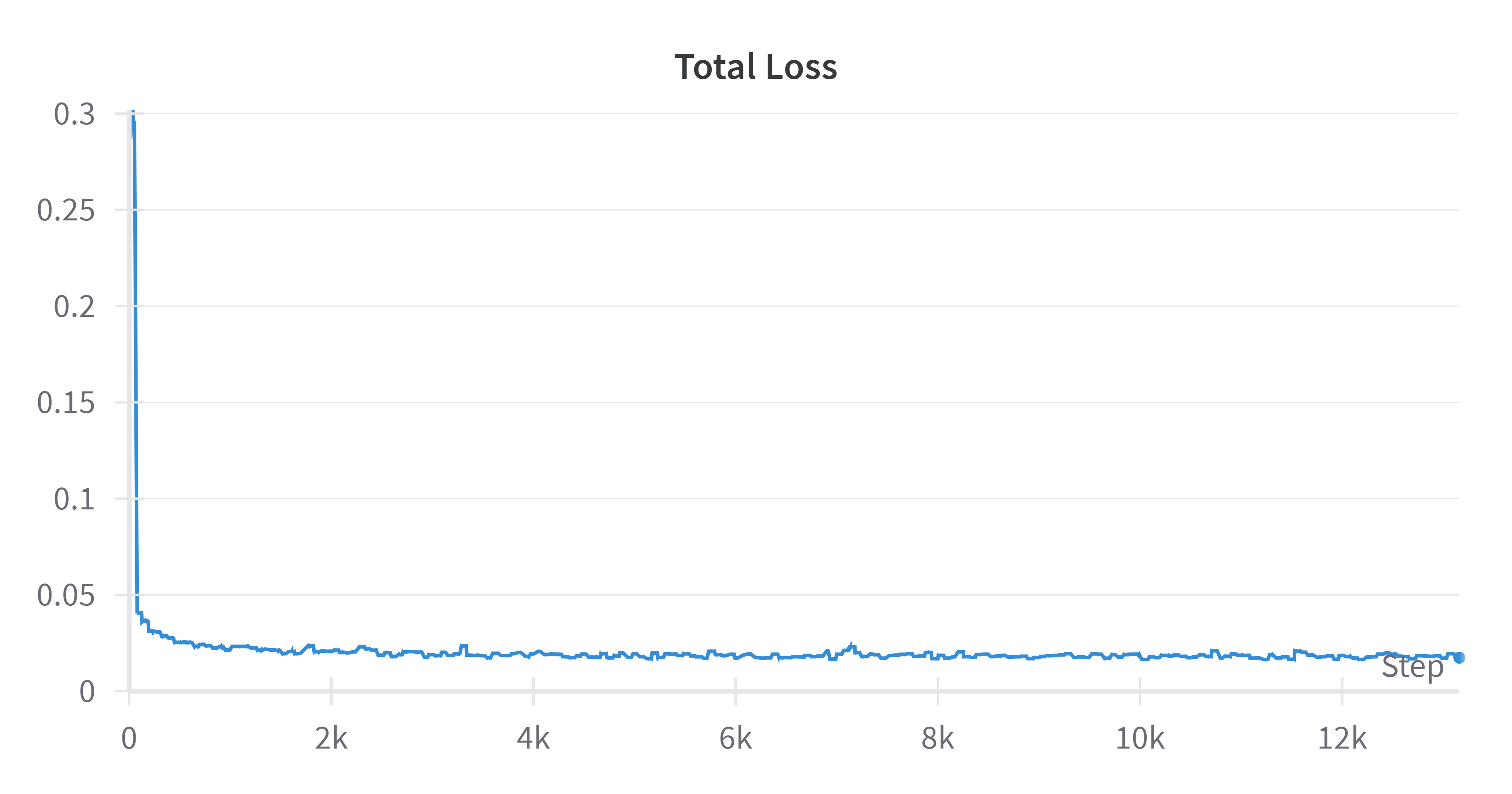
(total loss curve of an 1:8 autoencoder trained on Pythia-70m)

Do learned features consistently transfer between different model sizes and training datasets?

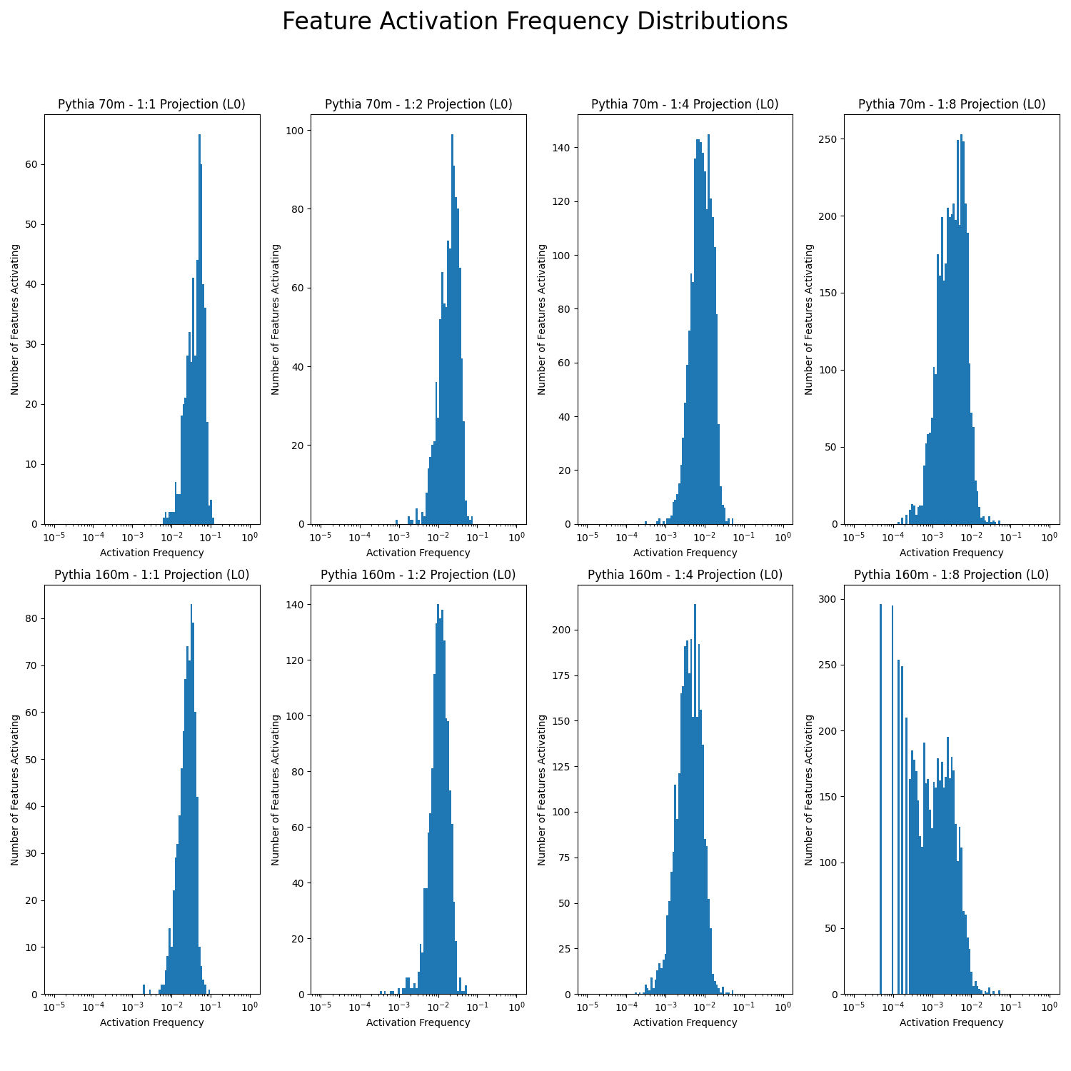
Activation frequencies are distributed roughly symmetrical around 0.01, meaning that the modal encoded neuron activated around once every one hundred tokens. This is solid evidence that our sparse autoencoders were effectively learning sparse, monosemantic representations. If a neuron was only needed every one hundred tokens to reconstruct the input, it likely represents a very specific concept rather than many concepts all at once. We see no clear trend when varying model size, demonstrating that this does not have much effect on an autoencoder’s ability to extract monosemantic features.

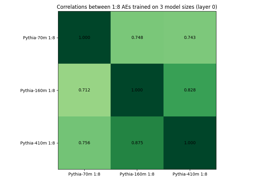
The table above measures the correlations between 1:8 autoencoders trained on layer 0 of three different model sizes. You can see that autoencoders trained on models closer in size have a higher correlation factor of their features, suggesting that smaller autoencoders may not store some of the features that large autoencoders do.

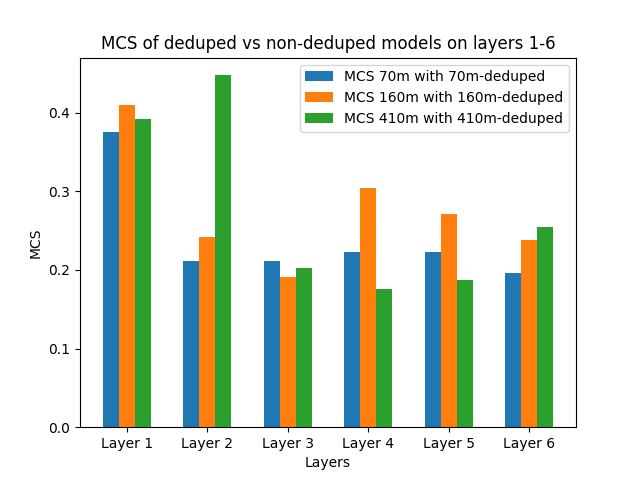
The above graph shows the MCS between autoencoders trained on deduped vs regular models. We anticipated the MCS of these models to be fairly high, but these were some of the lowest results we have seen, with autoencoders trained on layer 0 (of any of the three models we looked at) being around .4. Notably, all of our MCS were above .15 which was our baseline.

Are learned features consistent across different autoencoder sizes and training datasets?

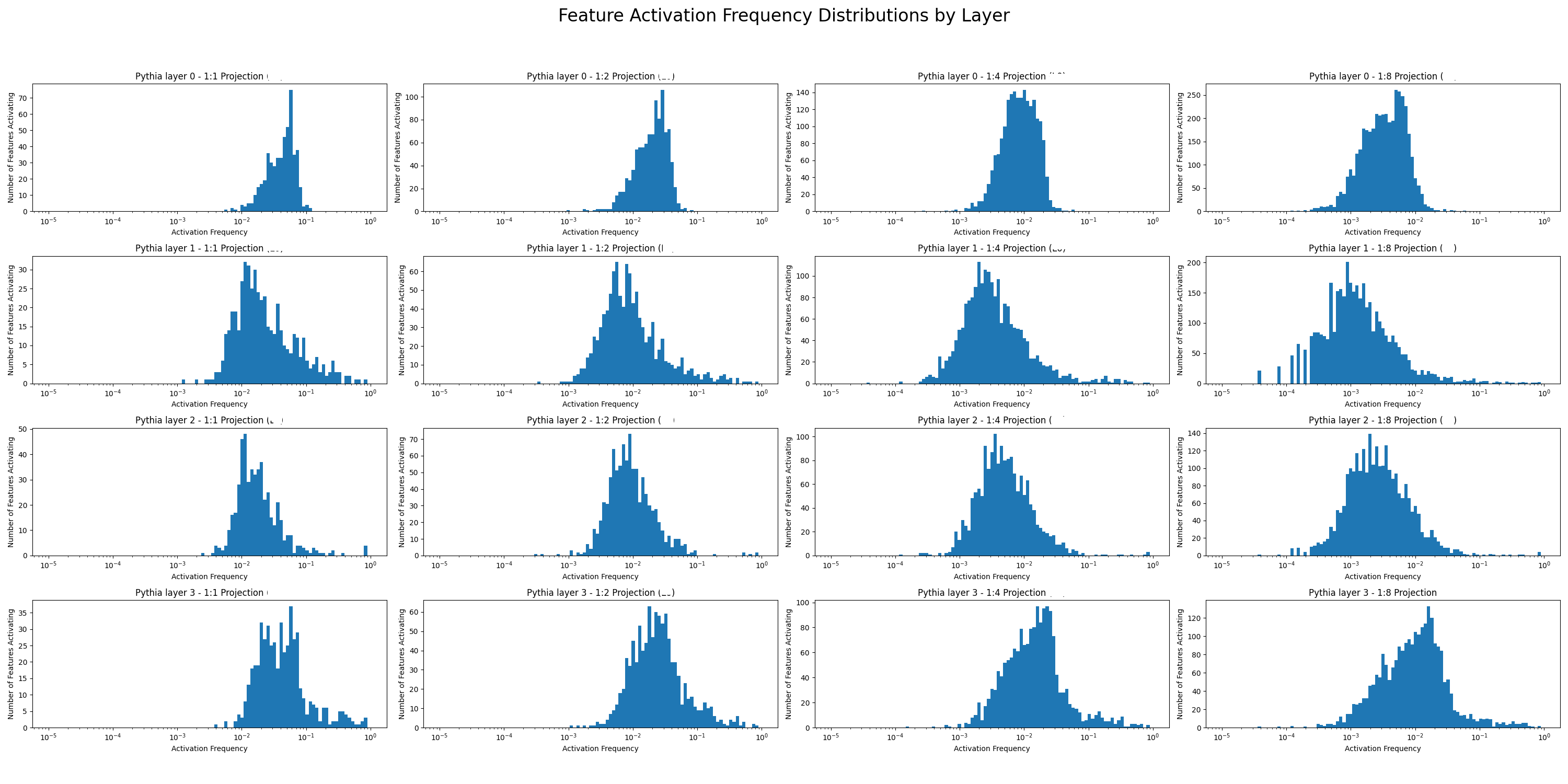
Sparsity tends to increase when the projection ratio increases, which makes sense, as a larger layer needs to use each neuron less often. This is evidence that our autoencoders are not learning all possible features, and using even larger autoencoders would allow us to unpack more features.

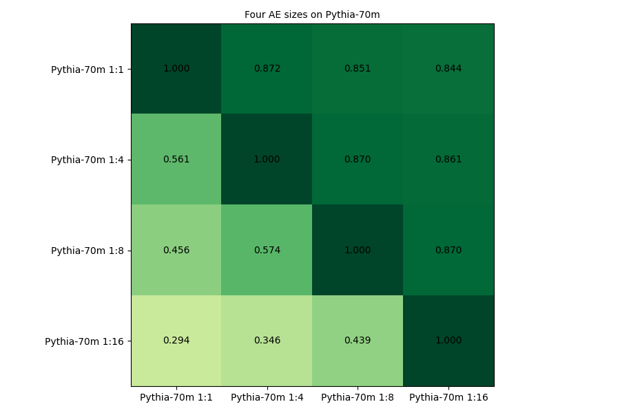
The above table looks at MCS loss of different sized autoencoders on Pythia 70m. Interestingly, we observed that MCS between autoencoders whose dimensions have the same ratio (e.g. 4:8 vs 8:16) are similar (e.g. both are .870.)

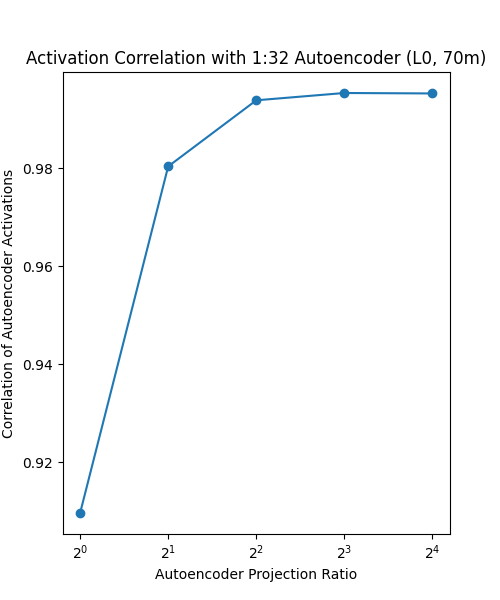
Activation correlations and MCS were very high for all autoencoder projection ratios, demonstrating that different size autoencoders learn very similar features. Note that all metrics were lower for the autoencoders with a 1:1 projection ratio, likely because they were penalized on sparsity while not having any additional space with which to represent concepts. This means the total information they could retain was likely much less than the other sizes. We see a slight upward trend as autoencoder projection ratio increases, which is small enough that it could probably be chalked up to the exact mean-max methodology used in the calculations. In the MCS graphs, the orange line represents mean-max MCS going from the smaller projection size to the larger projection size, where the blue line is the inverse. It is positive evidence that the blue line is much lower, because we should expect the most important features to correlate strongly with some of the features learned by the larger autoencoder, while the many features learned by the larger autoencoder should not all necessarily have a match in the smaller one.

Conclusion

Discussion

In this post, we explored the potential of sparse autoencoders as tools for interpreting neural networks, particularly focusing on their capability to disentangle polysemantic neurons into interpretable, monosemantic features. Our experiments, conducted on various configurations of Pythia models and sparse autoencoders, aimed to understand the consistency and universality of the features extracted by these autoencoders across different model sizes, training datasets, and autoencoder dimensions.

Our findings indicate that sparse autoencoders are indeed effective in learning sparse, monosemantic representations. This effectiveness is observed across different model sizes and is not significantly impacted by the size of the model, suggesting a level of universality in the features extracted. However, our results also reveal that the correlation between features tends to be higher in autoencoders trained on models closer in size, hinting at some limitations in the transferability of learned features across vastly different model scales.

Interestingly, we observed a tendency towards increased sparsity in the representations as we moved into the later layers of the network. This suggests that higher-level concepts in these layers might be more specialized and interpretable, aligning with intuitive expectations about neural networks.

Limitations

Limitations of sparse autoencoders include that they are extremely computationally intensive, especially if one wants to interpret multiple layers of a network, neural networks are not entirely human-interpretable to begin with, so their learned features will never quite represent human concepts, and all the metrics we use to analyze them rely on overall trends rather than individual features, so despite our ability to provide evidence to help answer broad questions, our analysis is still very imprecise.

Future Work

One future direction is focussing on training better sparse autoencoders, ones with lower reconstruction and sparsity loss. Given that we did not optimize our project for this and were limited by time and compute, it is very possible that better sparse autoencoders can improve our results.

It would also be interesting to train the same sparse autoencoder architectures on different datasets and see whether they are invariant to small perturbations in the dataset. If not, it’s evidence that the method may not work as well as we hope.

Finally, we could start to look at the features that the autoencoders are finding. We were able to measure similarity and correlations but did not have the time to look at the actual concepts that the representations were finding. This could give us additional insight into similarities between models that we currently are overlooking.

Acknowledgements

Special thanks to Sam Marks for suggesting the initial experiment ideas and to MIT AI Alignment for providing connections with mentorship and compute resources.