Analytic, Empirical, and Monte Carlo Bayesian Methods for Uncertainty Estimation
In the realm of machine learning, the robustness and reliability of predictive models are important, especially when confronted with Out-of-Distribution (OOD) data that deviate from the training distribution. Bayesian models stand out for their probabilistic foundations, being able to offer ways to quantify uncertainty. This project will present a survey of already-established methods of estimating uncertainty, as well as how we adapted/generalized them.
Motivation
Many practical uses of deep neural network (DNN) models involve using them with a restricted amount of training data, which doesn’t encompass all the potential inputs the model might face when actually used. This exposes a significant limitation of models based on data: they can behave unpredictably when dealing with inputs that differ from the data they were trained on, known as out-of-distribution (OOD) inputs. Machine learning models that are trained within a closed-world framework often mistakenly identify test samples from unfamiliar classes as belonging to one of the recognized categories with high confidence
Consequently, there has been a surge of research focused on improving DNN models to be able to assess their own uncertainty and recognize OOD inputs during their operational phase
Stochastic Weight Averaging Gaussian (SWAG)
SWAG
def train_swag(net, loader, num_epochs=5, K=25, swag_freq=50, swag_start=1):
    theta = get_all_weights(net)
    d = theta.shape[0]
    D = torch.zeros((d,K)).cpu()
    theta_bar = theta.clone().cpu()
    M2 = torch.zeros(d).cpu()
    sigmas = torch.zeros(d).cpu()
    optimizer = optim.Adam(net.parameters(), lr=0.001)

    net.train()
    for epoch in range(num_epochs):
        train_loss = 0
        n_ = 0
        for batch_idx, (data, target) in enumerate(loader):
            optimizer.zero_grad()
            output = net(data.to(device))
            loss = F.cross_entropy(output, target.to(device))
            loss.backward()
            optimizer.step()
            train_loss += loss
            if batch_idx % swag_freq == 0:
                if (swag_start <= epoch):
                    with torch.no_grad():
                        w1 = n_/(1+n_)
                        w2 = 1/(1+n_)
                        theta = get_all_weights(net).cpu()
                        theta_bar_new = w1*theta_bar + w2*theta
                        M2 = M2 + (theta-theta_bar)*(theta-theta_bar_new)
                        theta_bar = theta_bar_new.clone().cpu()
                        D[:,0:-1] = D[:,1:]
                        D[:,-1] = theta - theta_bar
                        sigmas = M2/(1+n_)
                        n_ += 1
    return theta_bar, sigmas, D
The learned \(\bar{w} \in \mathbf{R}^d\) is the mean of the posterior distribution on weights. The \(\Sigma\) vector represents the running variance of the weights and can be diagonalized to get a very rough posterior. (The method we used to determine the running variance is unlike the one presented in the SWAG paper due to issues with numerical instability and catastrophic cancellation which resulted in negative variances. To address this issue we used Welford’s online algorithm.) The \(D\) matrix contains the last \(K\) deviations of updated \(w\) values from \(\bar{w}\) (including the effect that the updated \(w\) has on \(\bar{w}\)). This allows us to form a rank \(K\) approximation of the posterior covariance. Thus we have the posterior \(P(w\mid\mathcal{D}) = \mathcal{N}\left(\bar{w}, \frac{1}{2}\left(\text{diag}(\Sigma) + \frac{DD^T}{K-1} \right)\right)\). To sample from the posterior, we do the following reparametrization
\[z_d \sim \mathcal{N}(0, \mathbf{I}_d)\] \[z_K \sim \mathcal{N}(0, \mathbf{I}_K)\] \[\tilde{w} = \bar{w} + \frac{1}{\sqrt{2}}\text{diag}(\Sigma)^{\frac{1}{2}}z_d + \frac{1}{\sqrt{2(K-1)}}Dz_K\]It is important to note that while a prior distribution on weights is not specified, it is implicitly chosen through how often we update our running average of the weights, variances, and deviations, as well as the optimizer being used.
For the purposes of inference, each \(\tilde{w}\) determines the parameters for a clone model and with \(S\) samples we effectively have an ensemble of \(S\) models. Their output distributions are averaged arithmetically to yield the final output. We expect that for in-distribution inputs, the individual outputs do not disagree drastically. And for out-of-distribution inputs, the individual outputs can differ a lot. So like with out other ensemble method, a good metric of uncertainty here is to use the average-pairwise KL divergence between the distributions. Here are some results and findings of this metric applied to SWAG.
We train a model with SWAG on the MINST and CIFAR10 datasets. First, we only train on the digits/classes from 0-5 and look at the KL scores on the digits/class 6-9. Expectedly, the scores tend to drastically increase on the unseen digits. However, the increase is less drastic for the CIFAR dataset as the data is a bit more homogenous.
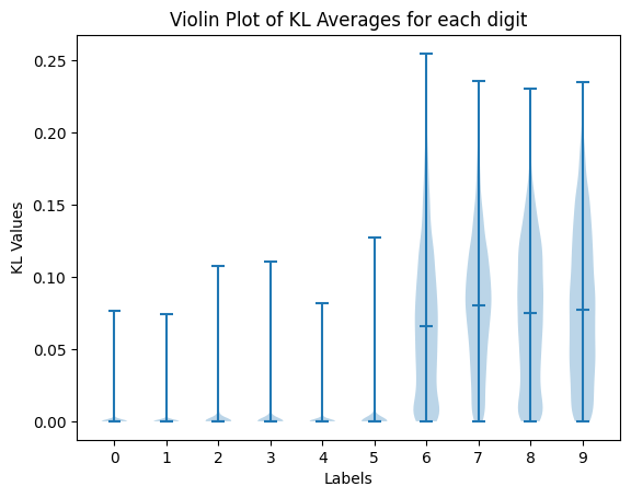
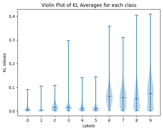
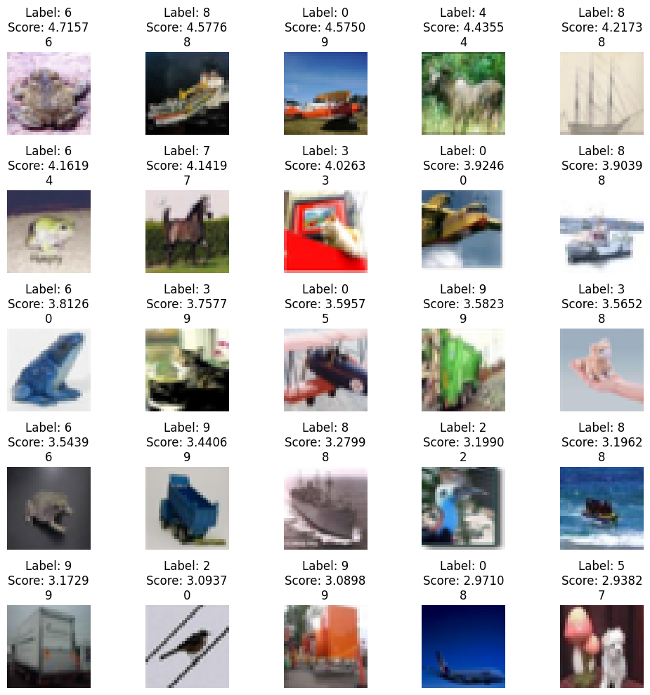
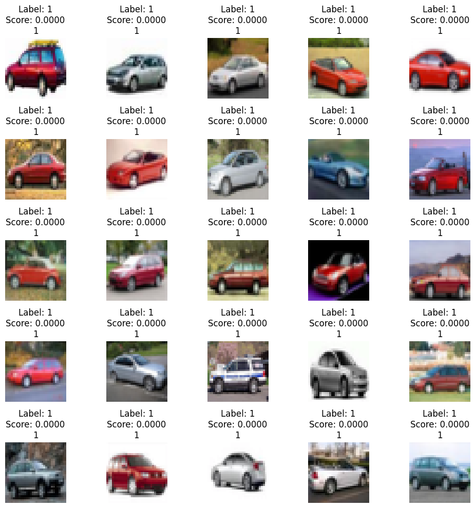
We can also take a look at the data itself and identify the images which have the highest and lowest scores for different splits of the data. For these images, we identify the true label, followed by the KL score assigned to the image (higher being more uncertain), and finally the predictions made by 10 of 25 sampled models.
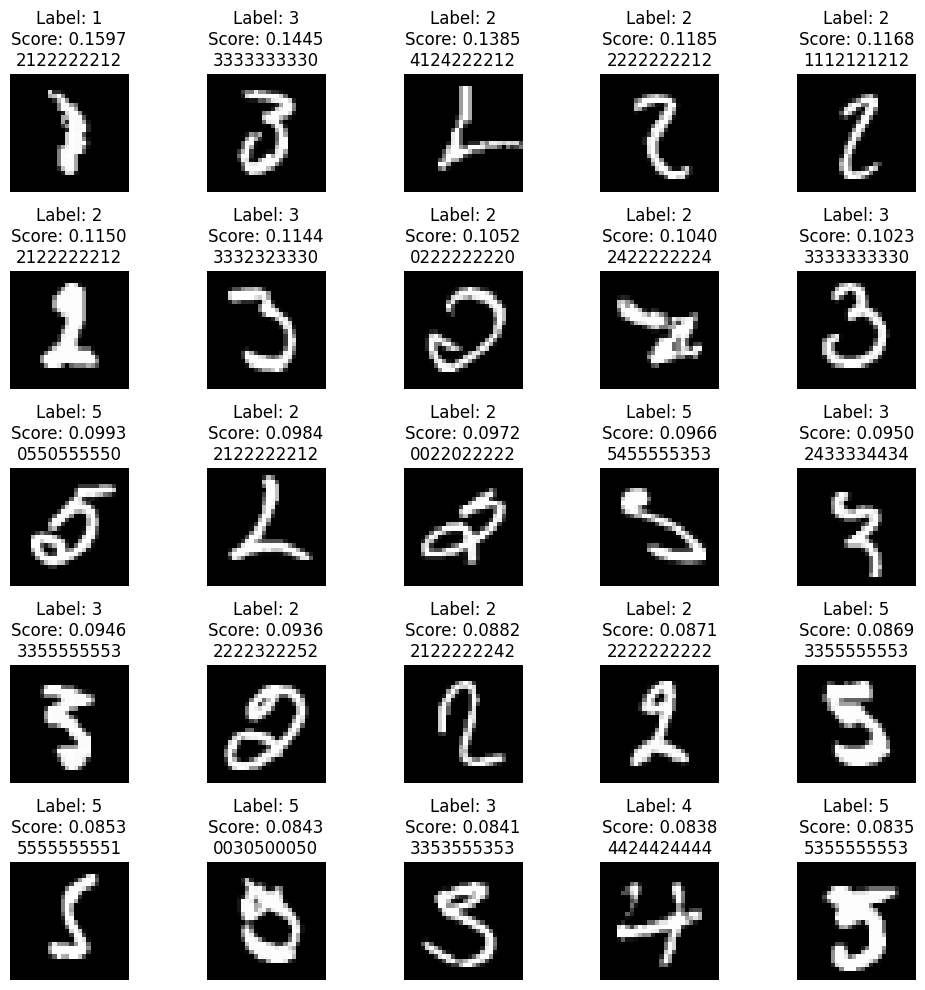
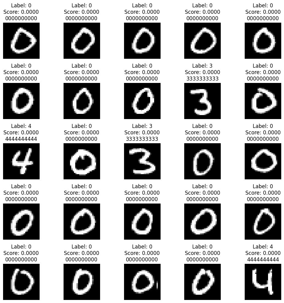
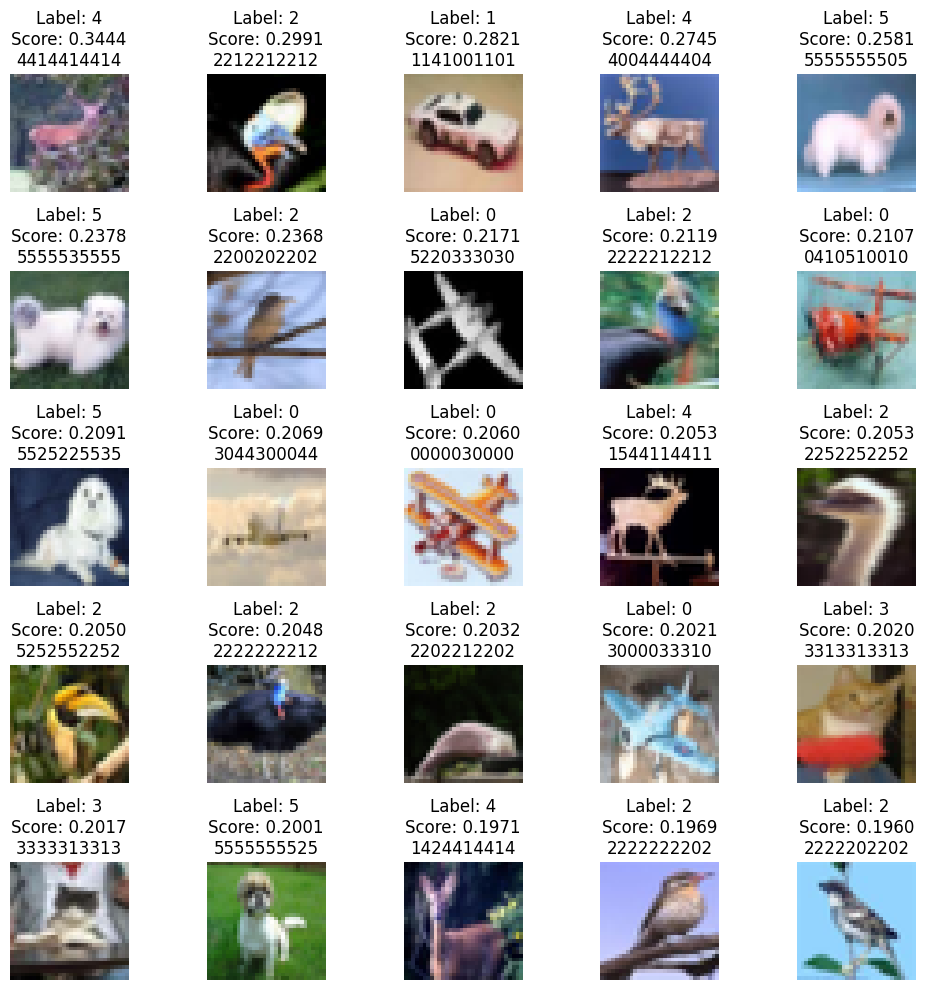
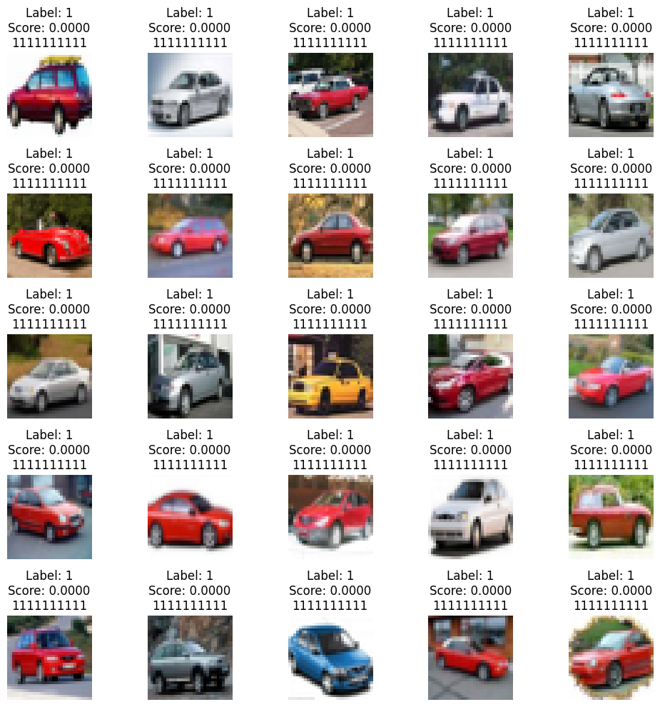
The above pictures correspond to the highest and lowest scores from in-distribution training data. The major contributors for the high scores for MNIST are digits that are so poorly written it’s hard to say what it is or it resembles another image too much. For CIFAR, it seems like the high score images are inducing confusion due to their color scheme or background. A lot of images with a blue or sky background such as those of birds do seem to be mistaken for planes at times. The low score images on the other hands are all extremely similar to one another; they’re very well written digits (usually 0) or something that is obviously a car (usually red).
Next, we take a look at how these scores fair on new out-of-distribution images.
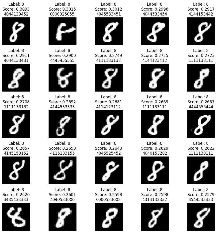
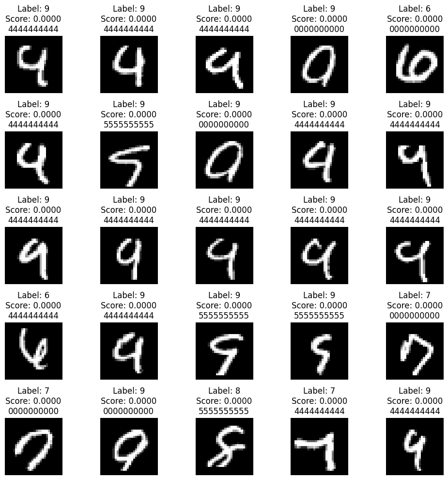
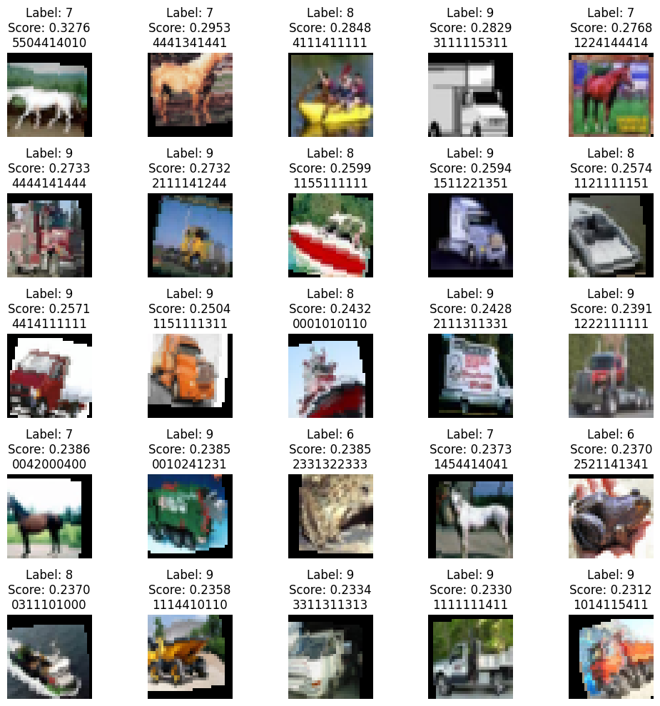
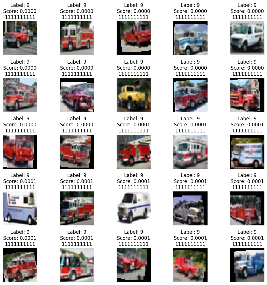
These are the highest and lowest scores on the OOD dataset. It’s unsurprising that the highest scores are assigned to the images that are unlike anything in the training set. For MNIST this is the number 8 and for CIFAR there doesn’t seem to be any one class. However, it is important to see that there are still images where our model has very low scores (high certainty). However, this simply comes from the fact that these inputs happen to look more similar to one class of training images (9 is really similar looking to 4 and trucks look pretty close to cars, especially if they’re red since a lot of the low score car-images are red).
All the methods used in this paper tend to show similar results for the images corresponding to the highest and lower measures of uncertainty so we won’t be lookig at those images for every single method.
Now that we’ve seen that we can use our measure of uncertainty as how well the output will yield the correct answer, we can try using uncertainty of output as a way to predict error. Ideally, we would like to see some sort of correlation between our uncertainty measure and our actual errors or probability of corect answer. So we retrained our models on all digits using SWAG and looked at the performance on a validation set. Notice that we don’t care too much about the error itself, but it’s (actually the probability of target label) correlation with the uncertainty measure. In particular, we look at the Spearman correlation to capture nonlinear relationships.
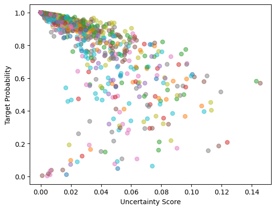
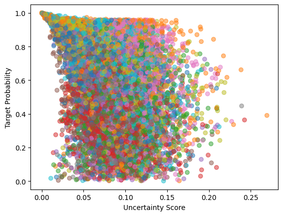
There is significant negative correlation which is what we’re looking for. If we can predict how well our model will perform on certain inputs, it allows us to better deploy model in real world situations as well as possibly improve it by doing something such as boosting or improved training. We now look to improve this relationship between error and uncertainty measure by finding better uncertainty measures.
Local Ensemble: Monte Carlo Dropout
We start off by comparing with a very simple method. Given a neural net with Dropout layers, and a new datapoint from test ID or OOD datasets, we output \(50\) different probabilistic distributions (rather than setting our model on evaluation mode, we keep the Dropout layers on), \(p_1, p_2, \ldots p_{50}\). Our uncertainty score is \(\text{Unc}(x) = \frac{1}{49\cdot 50}\sum_{i\neq j}D_\text{KL}(p_i\, \Vert \, p_j)\), i.e. the average KL divergence between any pair of distributions. The intuition is that, when the model shouldn’t be confident about a OOD datapoint, dropping weights (which can be seen as perburtabions) should change our output distributions significantly. This sensitiveness indicates lack of robustness and certainty.
This model is very simple and our weight “peturbations” are not too mathematically motivated in the sense of them coming from some justified posterior. However, it still provides a good baseline to compare against.
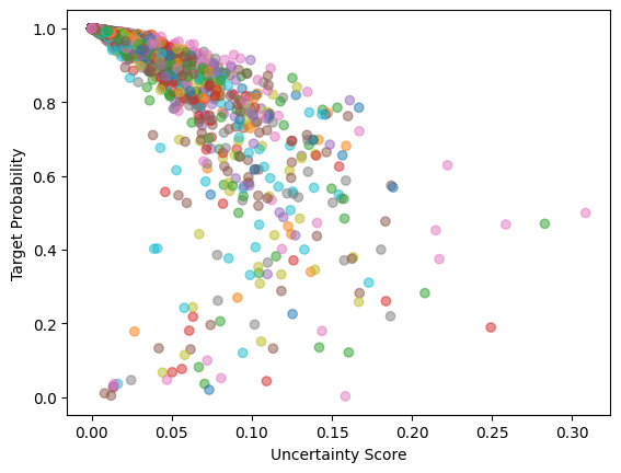
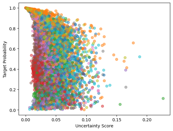
Overall, the error estimation on MNIST is about the same but significantly worse on the CIFAR dataset. This is about expected since MC dropout is such a simple method.
Sketching Curvature for Efficient Out-of-Distribution Detection (SCOD)
There is research literature on leveraging the local curvature of DNNs to reason about epistemic uncertainty. [Sharma et al.] explores this idea through a Bayesian framework. Let us assume a prior on the weights, \(P(w) = \mathcal{N}(0, \epsilon^2 I)\). By using a second-order approximation of the log-likelihood \(\log p(y,w\mid x)\), we arrive at the Laplace posterior \(P(w\mid\mathcal{D}) =\mathcal{N}(w^{MAP}, \Sigma^*)\), where \(\Sigma^* = \frac{1}{2}(H_L + \frac{1}{2\epsilon^2}I)^{-1}\) and \(H_L\) is the Hessian of the cross-entropy loss wrt \(w\). Given a pretrained DNN, \(\theta=f(x,w)\in\mathcal{R}^d\) where \(\theta\) determines a distribution on \(y\), we assume that the trained weights \(w^*\) are a good approximation for \(w^{MAP}\). We define our uncertainty metric to be the change in the output distribution, \(\theta\), when the weights are perturbed around \(w^*\) according to the posterior distribution. Using the KL divergence to measure distance between output distributions, we define
\[\text{Unc}(x) = \mathbb{E}_{dw\sim \mathcal{N}(0, \Sigma^*)}\left[ D_{\text{KL}}\left( p(\theta\mid x, w^*)\, \Vert \, p(\theta\mid x, w^* + dw)\right) \right]\]We can approximate the local KL divergence using the Fisher information matrix (FIM) of \(y\) wrt \(\theta\): \(D_{\text{KL}} \approx d\theta^TF_\theta(\theta)d\theta + O(d\theta^3)\). Also, by change of variables, we can rewrite the FIM in terms of \(w\): \(F_w(x, w) = J^T_{f,w}F_\theta(f(x,w))J_{f, w}\) where \(J_{f,w}\) is the Jacobian of the network outputs with respect to the weights. Putting this together, we get that
\[\text{Unc}(x) = \mathbb{E}_{dw\sim \mathcal{N}(0, \Sigma^*)} \left[dw^TF_w(x,w^*)dw \right] = \text{Tr}\left( F_w(x,w^*)\Sigma^*\right)\]We can also approximate \(\Sigma^* \approx \frac{1}{2}(MF_{w^*}^\mathcal{D} + \frac{1}{2\epsilon^2}I)^{-1}\), where \(F_{w^*}^\mathcal{D}\) is the averaged FIM on the training dataset
For simplicity, let us assume that the output of our DNN, \(\theta\), is the categorial distribution, i.e. \(\theta_i\) represents the probability assigned to class \(i\). In this case, we have that \(F_\theta(\theta) = \text{diag}(\theta)^{-1}\). Therefore, the FIM for one input os has rank at most \(\min(n, d)\) and we can represent it as \(F_w(x,w^*) = LL^T\), where \(L=J_{f,w}^T\text{diag}(\theta)^{-1/2}\). The same trick, however, doesn’t work for \(F_{w^*}^\mathcal{D}\) as it can reach rank as high as \(min(N, Md)\). For now, let us assume that we can find a low-rank approximation of \(F_{w^*}^\mathcal{D} = U\text{diag}(\lambda)U^T\), where \(U\in\mathbb{R}^{N\times k}\) and \(\lambda\in\mathbb{R}^k\). With a few mathematical tricks (which can be followed in [Sharma et al.]), one can prove that
\[\text{Unc}(x) = \epsilon^2\Vert L\Vert_F^2 - \epsilon^2 \left \Vert \text{diag}\left(\sqrt{\frac{\lambda}{\lambda + 1/(2M\epsilon^2)}}\right)U^TL \right \Vert^2_F\][Sharma et al.] also provides an randomized algorithm for finding \(U\) and \(\Lambda\) by using the FixedRankSymmetricApproximation
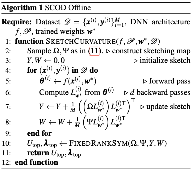
\(\Sigma\in\mathbb{R}^{r\times N}\) and \(\Psi \in \mathbb{R}^{s\times N}\) are random sketching matrices, which we chose to simply be matrices with i.i.d standard Gaussian entries. \(r+s\) is the size of the sketch and is ideally chosen as high as RAM allows. We also use the budget split \(s = 2k+1\) and \(r=4k+3\), where \(k\) is the target rank, as [Tropp et all.] suggests. We ended up setting \(k=50\) and got the following results:
We have been able to implement SCOD, but due to issues with saving our results and time, we can now only show the performance of the uncertainty score on predicting error on a subset (classes 0-5) of the CIFAR dataset.
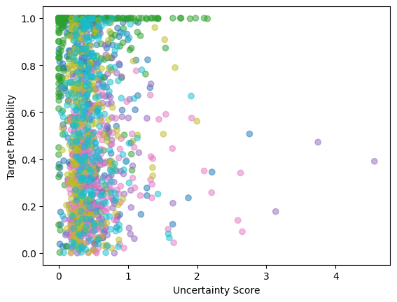
The score is a bit suspiciously low, so there may be something wrong with our implementation ignoring the fact that we only test of the subset. Nonetheless, it still a significant negative correlation and we get similar results when looking at high uncertainty and low uncertainty images.
SCODv2
We also did our own tweak on SCOD. Rather than having a vanilla prior, we can generalize it to any normal distribution with diagonal covariance. Let’s say that our prior is \(w\sim\mathcal{N}(0, \Sigma)\), where \(\Sigma\) is a diagonal matrix. Then, our Laplacian posterior’s covariance matrix becomes \(\Sigma^* = \frac{1}{2}(MF_{w^*}^\mathcal{D} + \frac{1}{2}\Sigma^{-1})^{-1}\). By the Woodbury matrix identity \(\Sigma^*=\Sigma - 2\Sigma U\left(\text{diag}(M\lambda)^{-1}+2U^T\Sigma U \right)^{-1}U^T\Sigma\). Using the well-known identities, \(\Vert A\Vert_F^2 = \text{Tr}(AA^T)\), \(\text{Tr}(AB) = \text{Tr}(BA)\), we get that
\[\text{Unc}(x_{\text{new}}) = \text{Tr}\left(\Sigma^*F_w(x_{\text{new}},w^*)\right) = \text{Tr}\left(L^T\Sigma L\right) - 2\text{Tr}\left(L^T\Sigma U\left(\text{diag}(M\lambda)^{-1}+2U^T\Sigma U \right)^{-1}U^T\Sigma L\right)\]\(= \left \Vert L^T \Sigma^{1/2}\right \Vert_F^2 - 2\left \Vert L^T \Sigma UA\right \Vert_F^2\), where \(AA^T = \left(\text{diag}(M\lambda)^{-1}+2U^T\Sigma U \right)^{-1}\).
Since \(\Sigma\) is a diagonal matrix, the biggest matrices we ever compute are of size \(N\times \max(k, d)\), which means that the computation is equally efficient asymptotically to the vanilla prior. To decide what diagonal matrix to use, for each layer, we assigned the same variance given by the variance of the weights of the same layer in a differently trained model (with same architecture).
Due to issues with saving our results and timing, we are not able to show our results estimating error from uncertainty for SCODv2.
Stochastic Curvature and Weight Averaging Gaussian (SCWAG)
Whereas SCOD attempts to analytically approximate the posterior by approximating the Hessian using the Gauss-Newton matrix, SWAG approximates the posterior by keeping running track of moments and deviations when it approaches flat regions in the loss landscape. What if we could combine these two ideas? We could use the SWAG emprical posterior. This method would not require matrix sketching of any form and lowers the required RAM necessary an SCOD can be quite RAM intensive. Using the \(\Sigma\) and \(D\) from SWAG to determine the posterior \(\Sigma^*\), we arrive the following measure of uncertainty (after digging through some math).
\[\text{Unc}(x) = \text{Tr}\left( F_w(x,w^*)\Sigma^*\right) = \frac{1}{2} \text{Tr}\left(F_w(x,\bar{w})\left(\text{diag}(\Sigma) + \frac{DD^T}{K-1} \right) \right)\] \[\text{Unc}(x) \propto ||L\Sigma||_F^2 + \frac{1}{K-1}||LD||_F^2\]We do this by introducing a wrapper model that takes in a base model as well as the SWAG outputs in order to perform the Jacobian based operations during each forward pass. For evaluation, we look at the Spearman correlation of the uncertainty score with the target probability and we notice some improvement over SWAG on the CIFAR dataset.
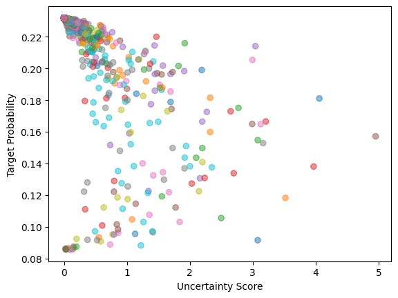
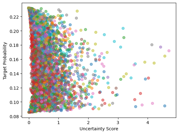
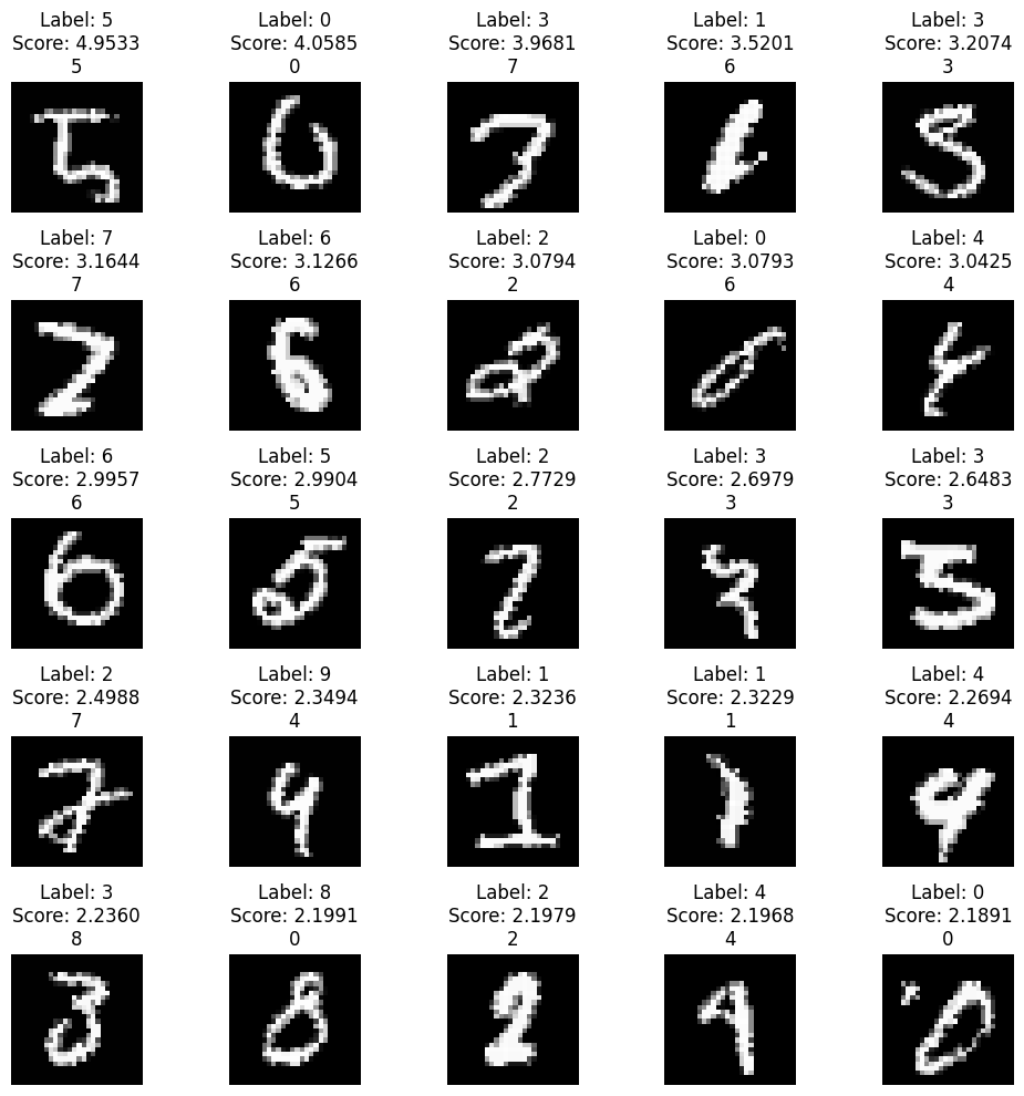
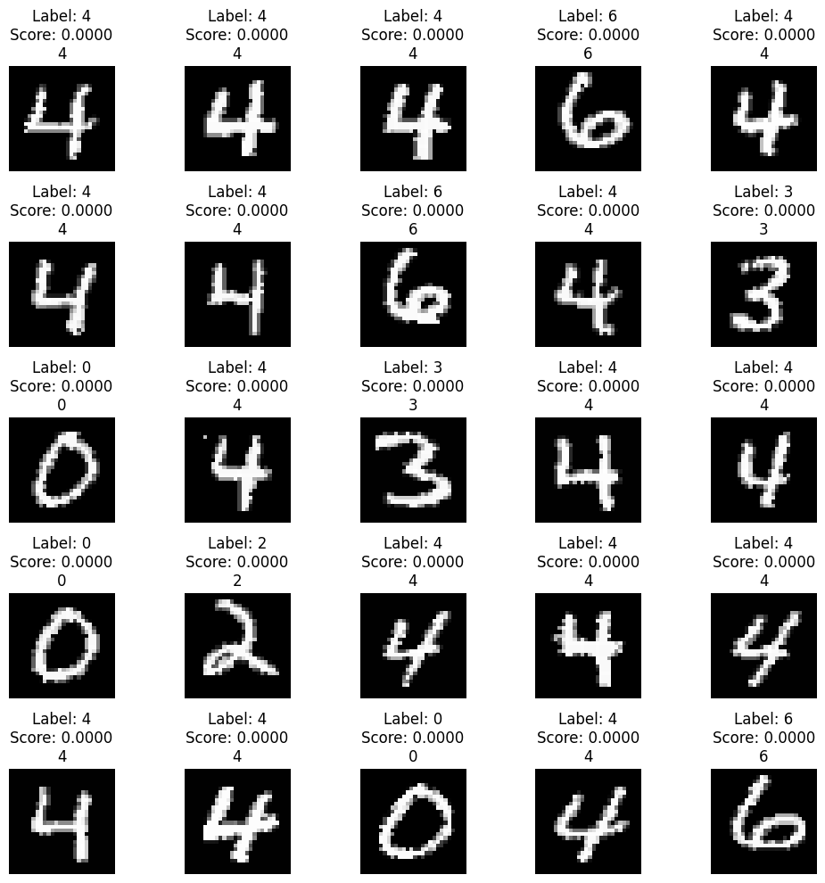
With MNIST, we already had near perfect correlation so this slight decrease isn’t too worrisome. However, the Spearman correlation has shot up drastically which shows that this method of combining the analytical approximation of uncertainty with an empirically constructed posterior has merit. There is something worrisome with the fact that the model with exactly \(bar{w}\) with its weights is producing distributions that have a maximum value of around \(.25\). We suspect we could have made some error here but have not been able to pinpoint anything wrong with out implementaton. The model still seems to have fairly accurate predictions as seen below.
Future Work
For SCWAG, we could work on figuring out why our output distributions becomes less spiked as a result of using \(\bar{w}\) as the weights for the network. We suspect that it’s a result of starting our SWAG averaging for \(\bar{w}\) too early so we were considering \(w\) far away from flat local minima of the loss landscape. Additionally, we could inspect the arcing nature in the plot of target probabilities vs score. For near 0 scores, it seems that the target probabilities arc from .25 to 0 which is unusual. Finally, we want to think of a way to introduce the loss landscape more into our approach. Maybe we can form a more expressive posterior. If we can manage that, our uncertainty estimates and correlation might improve. But more importantly, we would be able to call our method SCALL(y)WAG which is pretty cool.
In general and particularly for SCOD, we’d still like to experiment with priors that induce different types of posteriors. Because the dependence on prior is explicit here as opposed to implicit for SWAG, it allows us more room for experimentation in choosing nice expressive priors.