Predicting the Future: LSTM vs Transformers for Time Series Modeling
A comparison analysis between LSTM and Transformer models in the context of time-series forecasting. While LSTMs have long been a cornerstone, the advent of Transformers has sparked significant interest due to their attention mechanisms. In this study, we pinpoint which particular features of time series datasets could lead transformer-based models to outperform LSTM models.
6.S898 Final Project - LSTM vs Transformers for Time Series Modeling
By Miranda Cai and Roderick Huang

1. Introduction
In the context of time series forecasting, comparing Long Short-Term Memory (LSTM) networks to Transformers is a fascinating exploration into the evolution of deep learning architectures. Despite having distinct strengths and approaches, both LSTM and transformer models have revolutionized natural language processing (NLP) and sequential data tasks.
LSTMs, with their recurrent structure, were pioneers in capturing long-range dependencies in sequential data. While the accuracy of such models have been shown to be quite effective in many applications, training LSTM models takes a relatively long time because of the fact that they must remember all past observances. One faster alternative to LSTM models are transformers. Transformers are able to remember only the important bits of inputs using an attention-mechanism, and is also parallelizable making it much faster to train than recursive LSTMs that must be processed sequentially.
With its recent development, people have started opting to use transformer based models to solve sequence problems that once relied on LSTMs. One significant example is for NLP use cases, where transformers can process sentences as a whole rather than by individual words like LSTMs do. However, since transformers have been around for less than a decade, there are still many potential applications that are yet to be deeply explored. Thus, we will explore the effectiveness of transformers specifically for time series forecasting which finds applications across a wide spectrum of industries including finance, supply chain management, energy, etc.
Our goal is to realize which particular features of time series datasets could lead transformer-based models to outperform LSTM models.
2. Related Work
With the growth of ChatGPT in the recent years, extensive research has been done across various NLP tasks such as language modeling, machine translation, sentiment analysis, and summarization, each aiming to provide comprehensive insights into when each architecture excels and where their limitations lie. While research on time series data exists, it hasn’t garnered as much attention, so we aim to broaden this area of study.
2.1 Effect of Dataset Size
The size of a dataset plays an important role in the performance of an LSTM model versus a transformer model. A study

While we perform a similar methodology which is discussed further in section 4.1, the major difference is in the type of data we test. Instead of measuring classification accuracy for NLP tasks, this study measures the mean squared error (MSE) loss for regression time series data.
2.2 Effect of Noisy Datasets
Theoretically, LSTMs are more robust to noisy data due to its ability to capture local dependencies. On the other hand, the self-attention mechanisms in transformers propagate errors and may struggle with sequences that have a high degree of noise. Electronic traders have been recently attempting to apply transformer models in financial time series prediction to beat LSTMs
Financial data sets are known to be extremely noisy, and in addition, very hard to find due to their confidential nature. The application of
2.3 Effect of Multi-step Prediction
The last feature that we would like to look at between LSTMs and transformer models is forecasting length. Forecasting length describes how far into the future we would like our model to predict based on the input sequence length. One paper
Similarly to this paper, we will focus only on short-term forecasting. Short-term forecasting is important in situations like stock market predictions, where stock values show high volatility in the span of hours and may or may not have learnable trends over long periods of time.
However, we would like to extend the results of this paper to learn to also look at multi-step prediction. This study trained models specifically to have a singular output, with each model being trained with outputs at the specified prediction horizon. Instead, we would look to train our models against outputs of different lengths. We thought it would be an interesting addition to output the entire sequence of data leading up to whatever period in the future, to give a better visualization of what actually happens as forecasting length increases.
3. Methodology
The dataset we will be using throughout this study is the Hourly Energy Consumption dataset that documents hourly energy consumption data in megawatts (MW) from the Eastern Interconnection grid system
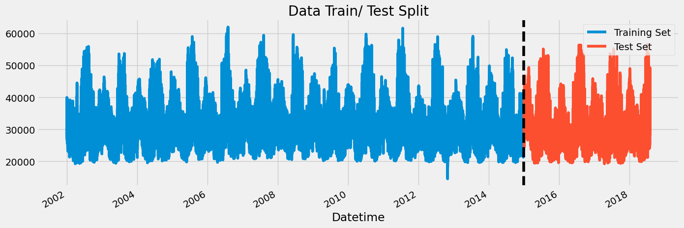
3.1 Experiments
We can utilize this dataset to predict energy consumption over the following features of a dataset.
-
Size of a dataset: As discussed in Section 2.1
, the size of a dataset played an impact in measuring classification accuracy for NLP tasks. Since the energy dataset is numerical, it’s important to test the same concept. We leveraged nearly 150,000 data points, progressively extracting subsets ranging from 10% to 90% of the dataset. For each subset, we trained the architectures, allowing us to explore their performance across varying data volumes. -
Amount of noise in the dataset: As discussed in Section 2.2
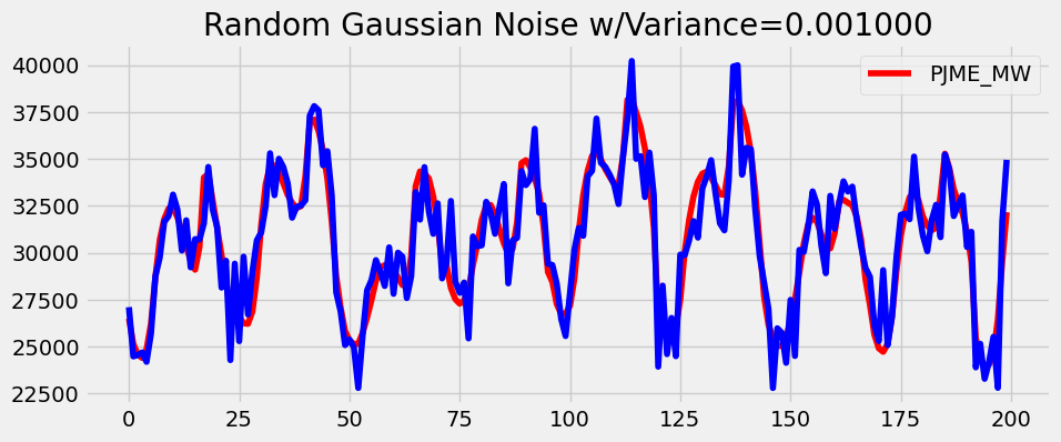
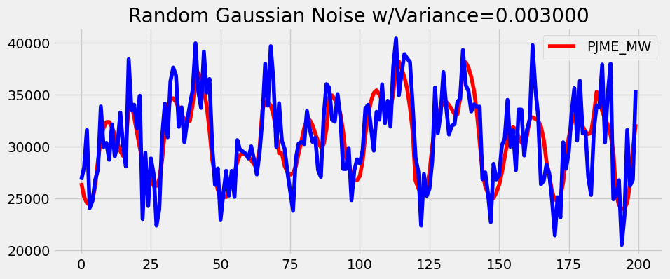
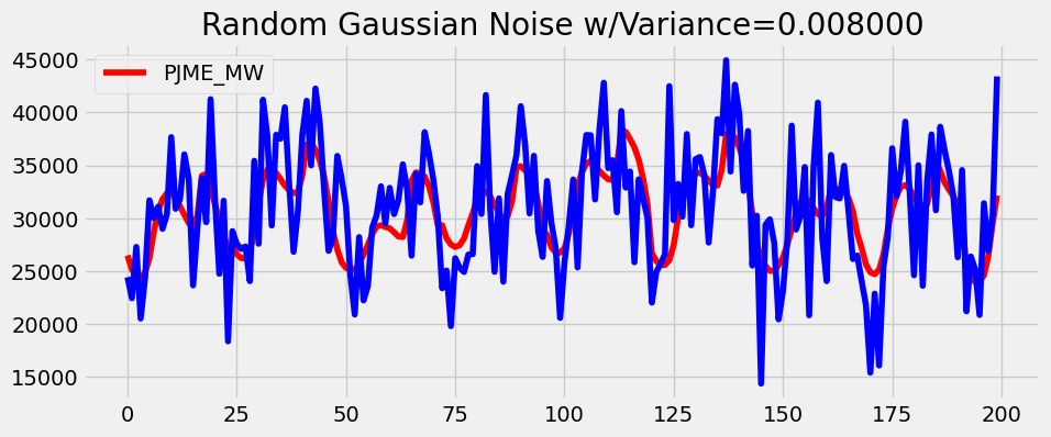
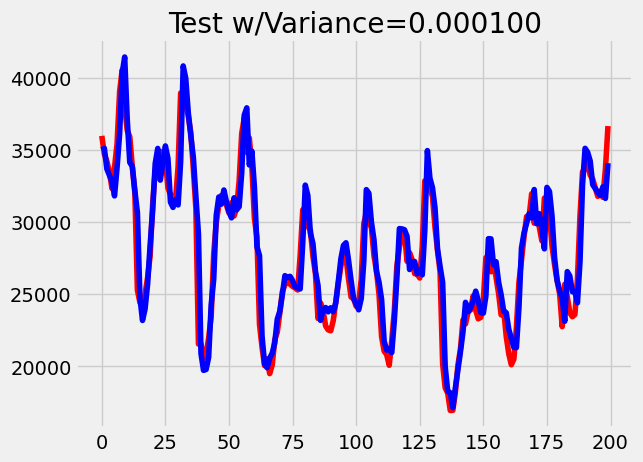
, research was done to test LSTMs vs transformers on noisy stock data for various assets. We deemed the energy dataset to be relatively clean since it follows a predictable trend depending on the seasons of the year and time of the day. For example, there are higher energy levels during the winter and daytime hours. To test noise, we added incrementing levels of jittering / Gaussian noise to observe the effect of noisy data on LSTMs and transformers. Example augmentations with different variances are plotted below in blue against a portion of the original dataset in red.

- Output size: As discussed in Section 2.3
, there have been few studies measuring the effect of varying the forecasting length, and in the ones that do they still only output one class at the specified time into the future. In our novel experimentation, we aimed to generate an entire sequence of outputs up until the specified time into the future. We created models that would predict forecasting lengths of 10%, …, 100% of our input sequence length of 10. To do so, we set the output size of our models to be equal to these forecasting lengths. This involved removing any final dense or convolutional layers.
3.2 Selected Architectures & Setup
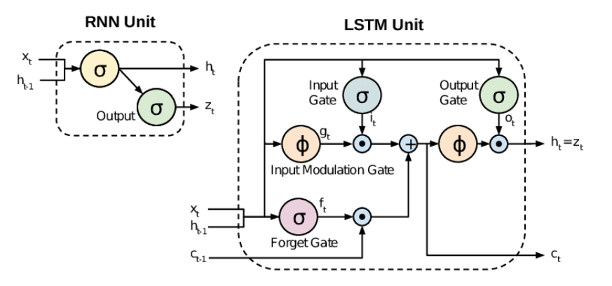
Selecting the right architecture for LSTM (Long Short-Term Memory) networks hinged on several key considerations. The LSTM architecture is extended of the RNN to preserve information over many timesteps. Capturing long-range dependencies requires propagating information through a long chain of dependencies so old observations are forgotten, otherwise known as the vanishing/exploding gradient problem. LSTMs attempt to solve this problem by having separate memory to learn when to forget past or current dependencies. Visually, LSTMs look like the following
Transformers, initially designed for natural language processing, should work well for time series data. They operate by utilizing self-attention mechanisms, allowing them to capture long-range dependencies effectively. A transformer breaks down the input sequence into smaller, fixed-size segments known as tokens, representing various time steps or features. Through multiple layers of self-attention and feedforward operations, the transformer architecture should excel at capturing both short-term and long-term dependencies. A figure of transformer time series is shown below from

There were certain parameters that we kept fixed throughout all variations of our models. The first was training on batches of data with sequence length 10. Second, we trained all of our LSTM models for 500 epochs and all of our transformer models for 10 epochs. These numbers were chosen with some fine-tuning to yield meaningful results while also allowing the training for so many individual models to be done in a reasonable amount of time.
Additionally, the data was normalized since the range of energy values was from 10000 Megawatts (MW) to 60000 MW. Normalizing the data improves convergence for gradient descent optimization and mitigates issues related to model regularization.
4. Experimental Results and Discussion
4.1 Size of a Dataset
Given the energy consumption dataset described in Section 3, we trained and evaluated an LSTM model and transformer model on progressively increasing subsets ranging from 10% to 90% of the dataset. The figure below shows the normalized mean squared error (MSE) loss for each subset of the dataset.
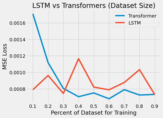
The experimental results show that transformers have an improving trend as the size of the dataset increases while the LSTM has an unclear trend. Regardless of the size of the training dataset, the LSTM doesn’t have a consistent result for the testing set.
In an LSTM, there exist additional gates for a sequence of inputs $x^{(t)}$ where in addition to the sequence of hidden states $h^{(t)}$, we also have cell states $c^{(t)}$ for the aforementioned separate memory. While the LSTM architecture does provide an easier way to learn long-distance dependencies, it isn’t guaranteed to eradicate the vanishing/gradient problem discussed in Section 3.2. While the same is true for transformers, the transformer architecture addresses the vanishing/exploding gradient problem in a different way compared to LSTMs. Transformers use techniques like layer normalization, residual connections, and scaled dot-product attention to mitigate these problems.
For time series dataset, the transformer architecture offers the benefit of the self-attention unit. In NLP, it’s typically used to compute similarity scores between words in a sentence. These attention mechanisms help capture relationships between different elements in a sequence, allowing them to learn dependencies regardless of their distance in the sequence. For time series data, transformers might offer advantages over LSTMs in certain scenarios, especially when dealing with longer sequences or when capturing complex relationships within the data such as seasonal changes in energy use.
From a qualitative perspective, if we pull a subset of the test data to observe the predicted values from an LSTM vs a transformer for 40% of the training set, we have the following.

While transformers did perform better than LSTMs, it’s not like the LSTM did a horrible job. We notice that at the peaks, the LSTM overshot more than the transformer and at the troughs, the LSTM undershot. However, overall, both architectures still had good results. In the context of the size of time series data, transformers do seem more promising given the loss figure above. It seems that LSTMs are losing that dependency on old observations while transformers are gaining ground as the size of the dataset increases. While
The performance of a model is dependent on the task and the data, and therefore before making a model choice, these factors should be taken into consideration instead of directly choosing the most popular model. - Ezen-Can 2020
For this experiment, the outlook of large datasets in time series applications for the transformer architecture looks promising.
4.2 Amount of Noise in a Dataset
To test the performance of our models on simulated noisy data, we first trained our models on batches of the original clean dataset and then ran our evaluations on different levels of noisy data. Random noise was added according to Gaussian distributions with variances in [0.0, 0.0001, 0.001, 0.002, 0.003, 0.005, 0.008, 0.01] to create these data augmentations. Below is a comparison of the MSE loss for both models as a function of the injected noise variance.
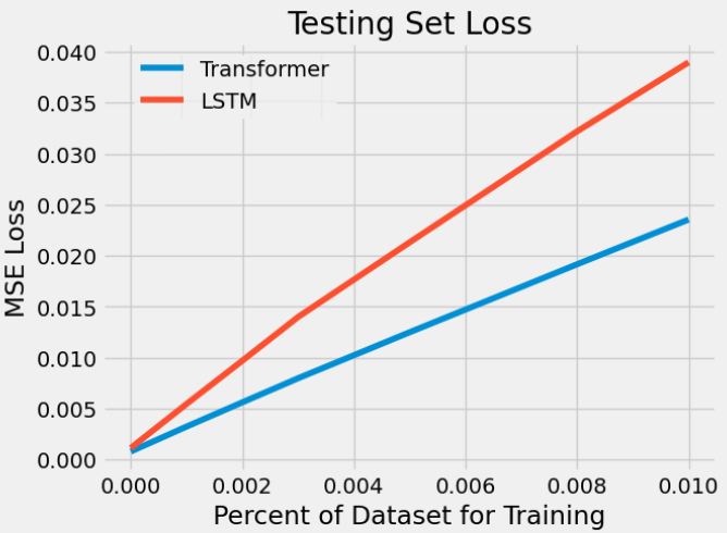
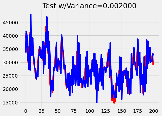
Since loss is not very descriptive in itself, we also visualize the model output for some of these augmented datasets. For each graph below, red is the true value while blue is predicted value.
| LSTM | Transformer |
 |  |
 |  |
 |  |
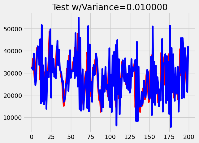 |  |
Both models are shown to start off similarly, predicting very well with no noise. However, almost immediately we can see that the LSTM does not handle noise as well as the transformer. LSTM makes much noisier predictions with many more outliers. We suspect this occurs due to the implicit inductive bias of the memory feature in the LSTM module. Consider a time step $t$. The memory accrued up to point $t$ “weights” the data seen in recent past time steps $t-1$, $t-2$, $\ldots$, much more so than the data seen relatively long ago. While this is an intuitive design for memory, we can observe that this mechanism combines storing temporal information with token-specific information. In order to compete with a transformer, the LSTM model needs to be trained on significantly more data.
The transformer on the other hand has the negative effects of its own inductive bias mitigated by its attention mechanism. Because the transformer has both a mechanism to account for temporal information and a mechanism to select the next associated token (attention module), and because they are separated, it is able to produce more “accurate” results.
4.3 Prediction Size
Finally, we created and trained separate models with varying numbers of output classes to represent the prediction size. We trained on output sizes as percentages of our input size, in increments of 10% from 0% to 100%. Because our input sequence was a constant 10 and our data is given in hourly intervals, these percentages translated to have prediction horizons of 1hr, 2hrs, …, 10hrs. Evaluating our models resulted in the following MSE loss trends.

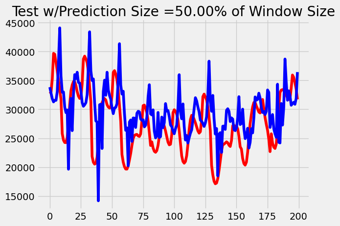
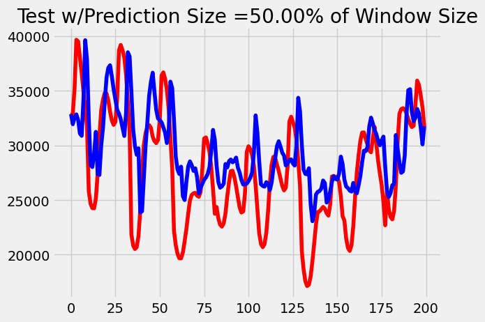
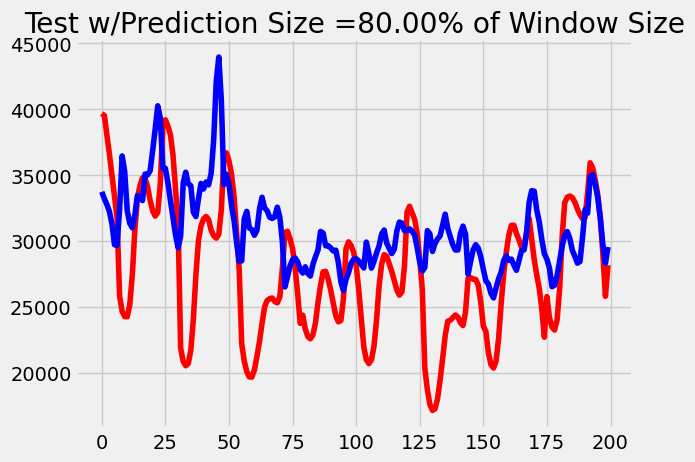
Again, to get a better sense of why we see these results, we visualize the outputs. Since our outputs are sequences of data, to have a more clean visualization we plot only the last prediction in the sequence. For each graph below, red is the true value while blue is predicted value.
| LSTM | Transformer |
 |  |
 |  |
 |  |
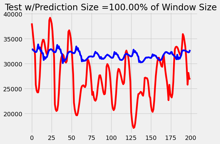 | 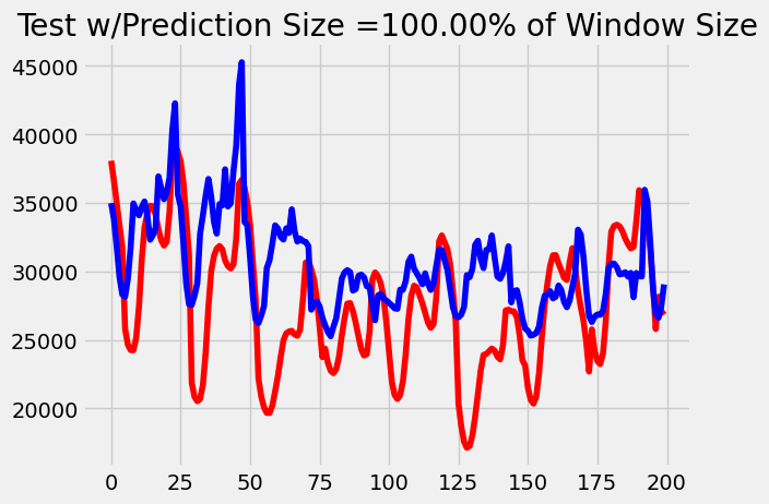 |
As we can see, the MSE loss of our transformer model increased at a slower rate than our LSTM model. After comparing the outputs of our models at these time steps, it becomes evident that this trend is due to the LSTM losing characteristic over time. Our transformer simply performs worse when it has to predict more as expected because the data is not perfectly periodic. However, we infer that the LSTM outputs get flatter over time because the more we accumulate memory through the long-term mechanism, the less weight each previous time step holds, diluting the total amount of information carried through the sequence. Transformers avoid this problem by using their attention mechanisms instead to keep only the important information throughout.
5. Conclusion
Through the experiments tested in Section 4 (on dataset size, dataset noise, and prediction size), transformers seem to be a promising alternative to LSTMs for time series modeling due to their unique architecture, particularly suited for capturing long-range dependencies. Unlike LSTMs, transformers utilize self-attention mechanisms that allow them to consider relationships between all elements in a sequence simultaneously. This capability is especially advantageous in time series data, where capturing distant dependencies is crucial for accurate forecasting. Additionally, transformers mitigate vanishing gradient problems better than LSTMs, enabling more robust training on longer sequences.
While transformers excel in parallel computation theoretically, one significant issue is the extensive memory requirements during training, especially with larger models or datasets. Transformers demand significant memory for storing attention matrices, limiting the batch size that can fit into GPU memory. So, for those who are finding an optimal architecture to train a time series dataset, one has to consider his or her own design priorities of accuracy and performance.
All in all, the choice between LSTMs and transformers for time series datasets depends on the implementer’s design priorities and the task at hand. With some research showing LSTMs outperforming transformers and others such as our study showing the opposite, there is a clear need to dive deeper into the subject especially given the extensive number of applications for time series modeling.