Embeddings for Spatio-temporal Forecasting
An analysis of various embeddings methods for spatio-temporal forecasting.
Introduction
Time series forecasting is an interdisciplinary field that affects various domains, including finance and healthcare, where autoregressive modeling is used for informed decision-making. While many forecasting techniques focus solely on the temporal or spatial relationships within the input data, we have found that few use both. Our goal was to compare two SOTA spatiotemporal models, the STAEformer and the Spacetimeformer, and determine why one works better than the other. The papers on both models did not feature each other in their benchmark evaluations, and we thought that analyzing their embeddings and identifying their failure modes could offer new insights on what exactly the models are learning from the dataset. We hypothesized that the Spacetimeformer would perform better as its proposed approach, sequence flattening with Transformer-based processing, seems to offer a more flexible and dynamic representation of spatiotemporal relationships that doesn’t depend on predefined variable graphs. We focused on forecasting in the field of traffic congestion, which is a pervasive challenge in urban areas.
Related Work
We focused on two SOTA spatiotemporal models that were evaluated on traffic forecasting datasets. The first is the STAEformer

The second is the Spacetimeformer

Dataset
We used the PEMS08 dataset
Methodology
The problem statement is as follows: given the sensor readings across the 170 sensors for the previous N timesteps, we want to predict their readings for the next N timesteps. We tested the model with varying context lengths, but we found that the default value of 12 given in the STAEformer paper provided enough information to the model. We used huber loss as we wanted the model to converge faster in the presence of outliers, which was necessary given the limited compute that we had (training 50 epochs took around 3 hours).
We trained STAEformer for 50 epochs, which was sufficient to achieve performance metrics similar to that of the paper. To compare the embeddings from Spacetimeformer, we retrained the model end to end after replacing the embedding layer in the model with Spacetimeformer’s embedding layer. To do this, we kept the context dimensions the same and flattened the input sequence along the input dimension and the dimension corresponding to the number of sensors. This structured the embedding layer so that it could learn the spatiotemporal relations across the sensors from different time frames.
Replacing the embedding layer within the STAEformer with a pretrained embedding layer from the Spacetimeformer instead may seem like a more legitimate method to test the effectiveness of the embeddings, as we would basically be doing transfer learning on the embedding layer. However, the pretrained embeddings from Spacetimeformer might have been optimized to capture specific spatiotemporal patterns unique to its architecture, which was why we believe training the model end to end with the Spacetimeformer embeddings would result in a more accurate and contextually relevant integration of the pretrained embeddings into the STAEformer framework.
After training, we wanted to provide visualizations of the embeddings from STAEformer and Spacetimeformer to show whether the learned embeddings are meaningful at all. To do this, we obtained the embeddings by passing in the raw data through the embedding layers of the loaded models and generated t-SNE plots with them. For the STAEformer, we focused solely on the adaptive embeddings as they were the parts of the embedding layer that captured spatiotemporal relations in the data. To generate the t-SNE plots, we had to reshape the embeddings so that they could be passed into the function so we flattened them across the model dimension. After fitting the t-SNE, we then unflattened the embeddings back to their original shape and plotted them. Each sensor was color coded with different colors, and the results can be shown in the next section. We hypothesized that the t-SNE plots would contain clusters grouped by either the sensors or the time the readings were recorded.
After generating the t-SNE plots, we wanted to test the effects of perturbing the raw data on the embeddings. We wanted to know how the embeddings would change. For example, regardless of what the clusters represent, are they tighter? Will additional clusters be formed? Conversely, will some of the existing clusters break apart? In particular, we were hoping that augmenting the data would perhaps improve cluster formations in the worse looking embeddings, as there is a good possibility that the data itself isn’t good enough.
Results
The table below shows the results after training STAEformer and the STAEformer model with a Spacetimeformer embedding layer for 50 epochs each. Table of loss values:
| Embedding Layer | Train Loss | Validation Loss |
|---|---|---|
| STAEformer | 12.21681 | 13.22100 |
| Spacetimeformer | 12.42218 | 16.85528 |
We can see that the STAEformer had better training and validation loss than the Spacetimeformer. While the train loss converged to similar values, the validation loss for the model using the STAEformer embedding layer was much better. So now that we know the STAEformer embedding layer seems to perform better than the Spacetimeformer embedding layer, we plotted the embeddings for both to analyze why this is the case. To do this, we passed a data point from the validation set through the embedding layer. The results are shown in the figure below.
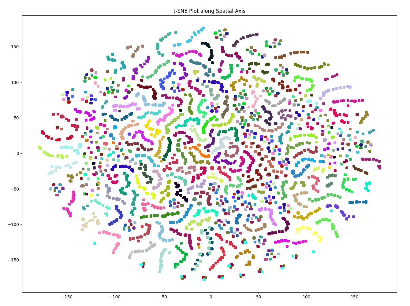
The t-SNE plot for the STAEformer embeddings shows clearly separate clusters for most of the 170 different sensors. The shape of each cluster is a “snake-like” trajectory. Therefore, we know that the embeddings preserve some pattern-like notion across readings from a single sensor. We hypothesize that each of these trajectories represent the reading of a single sensor over time. There are a couple outliers, where the clusters are not grouped by color. One prominent example is the string of cyan, maroon, and moss points along the bottom of the plot. However, even these points have some clustering, though they may not be clustered by color.
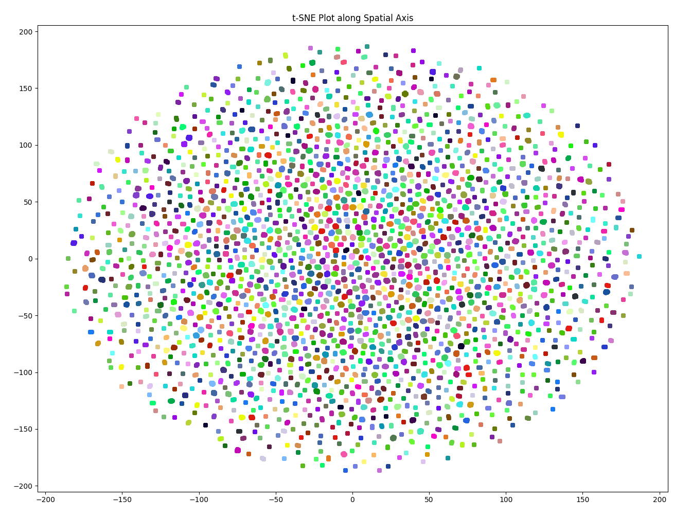
On the other hand, the t-SNE plot for the Spacetimeformer embeddings show no clear clusters across the same sensor. The distribution resembles a normal distribution, meaning that there is little pattern preserved in the embeddings. It becomes more difficult to differentiate between data points from the same sensor across time.
In order to further analyze the effectiveness of each embedding layer, we perturbed the training data and re-trained each model. We were expecting the clusters from the STAEformer embeddings to remain largely the same, with some of the existing clusters possibly breaking apart due to the added noise. However, we were hoping that the Spacetimeformer embeddings would show more visible clusters after the raw data was perturbed. Given the characteristics of the embeddings, one possible output we expected were clusters containing multiple colors. An example is shown in the following image.
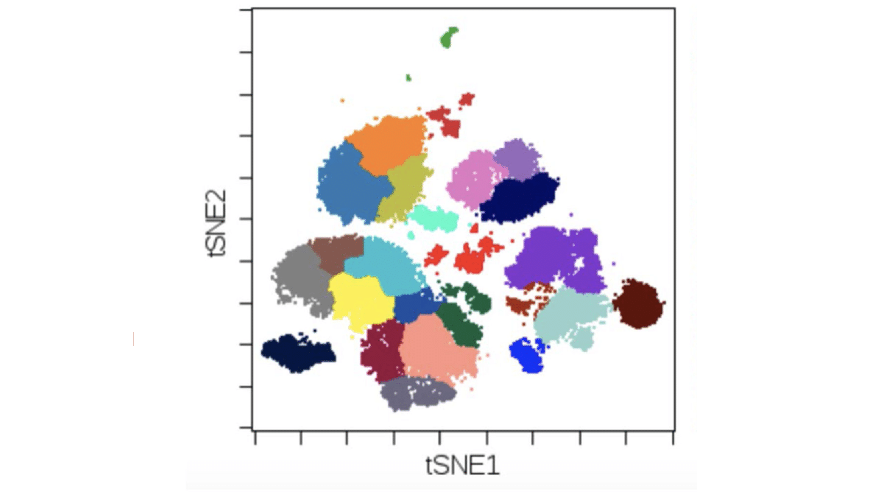
This would show that the Spacetimeformer successfully learned spatial relationships across the sensors at variable timesteps. Instead of each cluster representing the embeddings for one sensor, the presence of larger clusters with multiple colors could imply that the Spacetimeformer learned spatiotemporal relations among the corresponding sensors and embedded them into a larger cluster.
The following table shows the results after training the model with the perturbed data.
| Embedding Layer | Train Loss | Validation Loss |
|---|---|---|
| STAEformer (with perturbations) | 13.58251 | 13.35917 |
| Spacetimeformer (with perturbations) | 13.42251 | 17.01614 |
As expected, validation loss slightly increased for both models, and the STAEformer continued to have lower loss values than the model with the Spacetimeformer embedding layer.
When we generated the t-SNEplots with the new embeddings, we obtained the following:
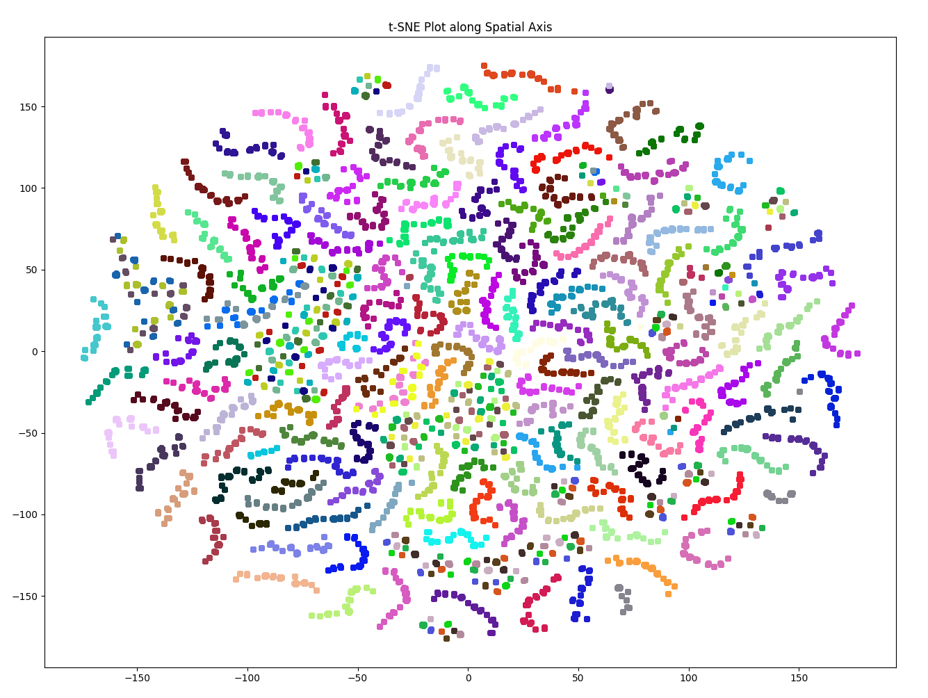
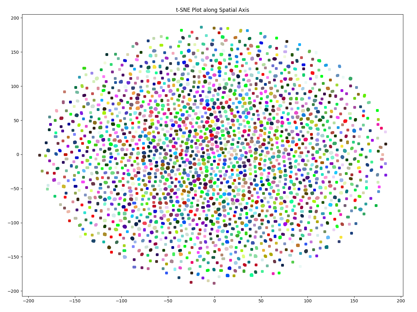
Both t-SNE plots for the STAEformer and Spacetimeformer embeddings look the same as when the models were trained on the original, unperturbed data. So unfortunately, the augmentation had little to no effect on the embedding layers for these two models.
Since the t-SNE plots can be hard to parse with the human eye, we decided to focus on the embeddings for the most relevant features of the dataset and see how they compared between the Spacetimeformer and STAEformer. In parallel, this would enable us to identify the failure modes of the dataset and augment those features to see if they improve the model performance. In order to do this, we used PCA to identify the principal components. From there, we found which features help explain the most variance in the dataset and identified those as the features that had the largest impact on the learned embeddings.
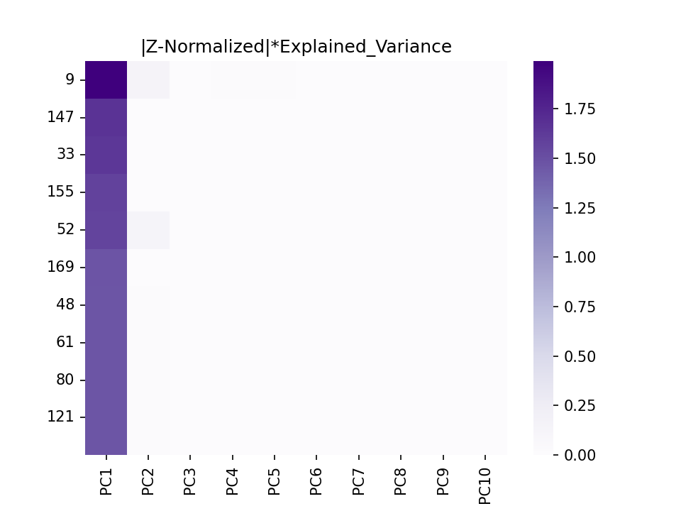
This heatmap shows the top 10 principal components and and the top 10 features that correlate with each principal component. From this heatmap, we can see that the 9th sensor in the dataset is the most relevant feature. Therefore, we can find the corresponding embedding to be the most relevant.
Using only the 5 most relevant embeddings obtained from PCA, we re-graphed the t-SNE plots. This helped us to narrow our attention to the most important embeddings.
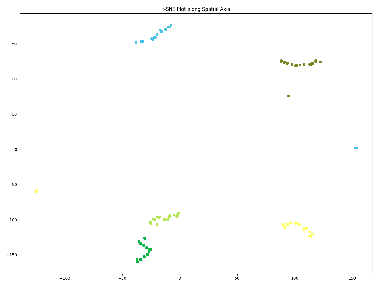
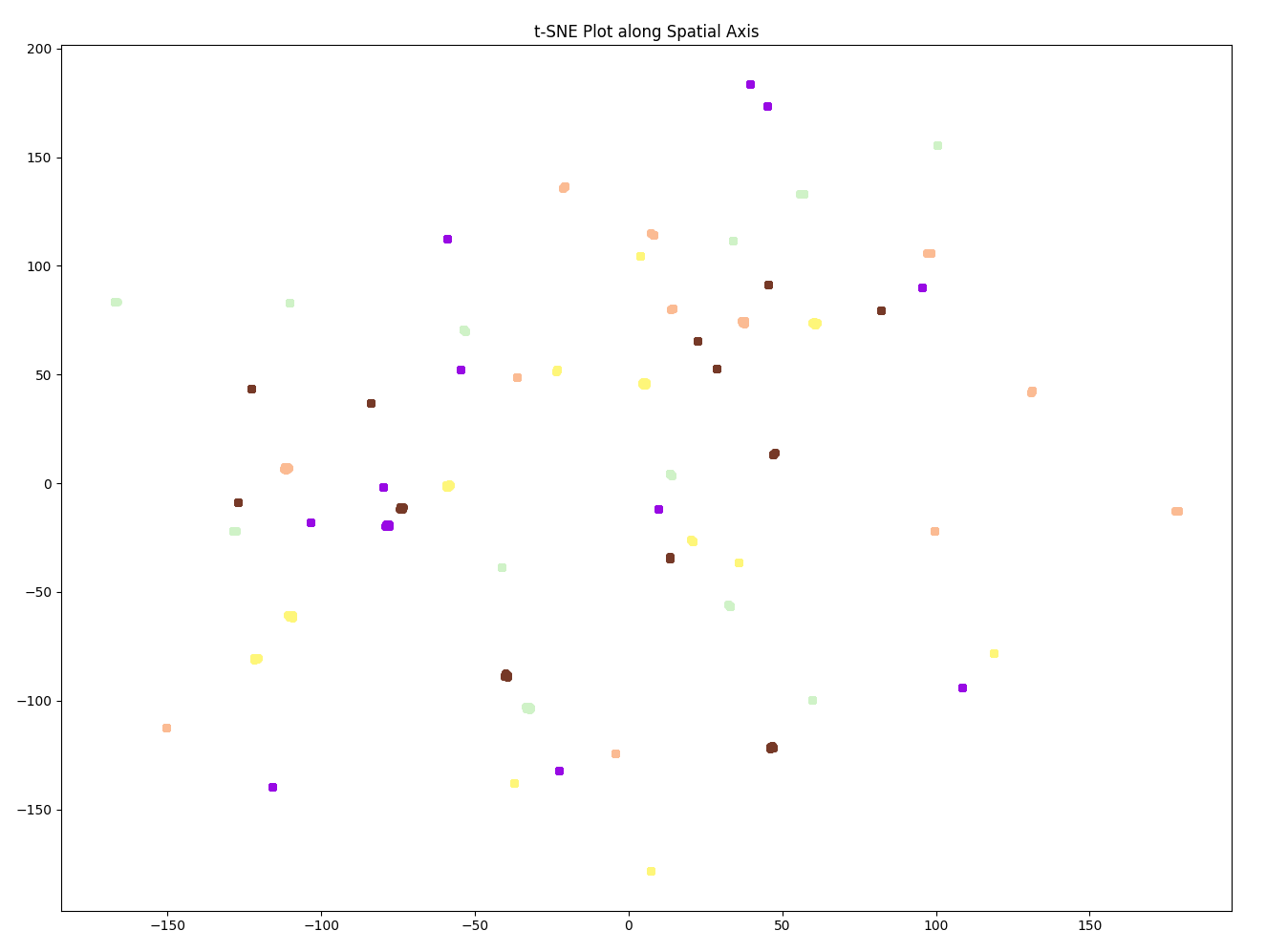
As expected, the embeddings for the most relevant sensors in the STAEformer all maintain the “snake-like” trajectory. However, the embeddings for even the most relevant sensors in the Spacetimeformer are seemingly random, and have no pattern across the points.
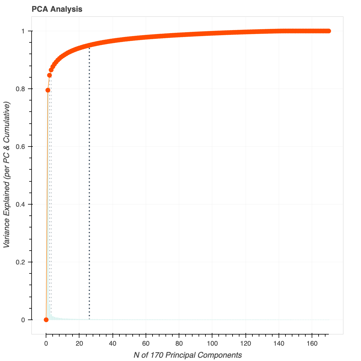
We found that the top 25 sensors explained 95% of the variance in the dataset, so we did a quick experiment where we augmented the rest of the 145 sensors (as opposed to the entire training dataset) to see how that affected the learned embeddings. For this augmentation, we expected the results to not improve by much since the learned embeddings for even the most relevant sensors in Spacetimeformer didn’t form visible clusters in the t-SNE plots. As expected, the results were almost identical to the ones generated from augmenting the entire dataset.
Conclusion, Discussion, Next Steps
There are a couple of reasons why we think the Spacetimeformer performed worse than the STAEformer overall. The first explanation that came to mind is that the readings across different sensors may be mostly independent from one another. The color coded t-SNE plots for the STAEformer clearly separate each sensor into its individual cluster. In this case, the Spacetimeformer would not be suited for the task as its embedding layer solely focuses on learning spatiotemporal relationships, while the STAEformer also contains an embedding layer that is solely dedicated to learning temporal relationships.
A second, more plausible explanation deals with the embedding architecture. The difference in performance between the STAEformer and the Spacetimeformer in time series forecasting shows the importance of adaptive embeddings in capturing spatio-temporal relationships. While the STAEformer introduces adaptive embeddings to comprehend the patterns in the data, the Spacetimeformer relies on breaking down standard embeddings into elongated spatiotemporal sequences. The t-SNE plots show that the STAEformer’s adaptive embeddings generate clusters representing sensors with snake-like trajectories, providing a visualization of the model’s ability to capture spatio-temporal patterns. In contrast, the Spacetimeformer’s embeddings follow a scattered distribution, indicating challenges in identifying clusters. This suggests that the Spacetimeformer’s approach may face limitations in effectively learning the spatio-temporal relationships within the PEMS08 dataset, and potentially traffic data in general.
Having said all this, the resilience of both the STAEformer and Spacetimeformer to perturbations in the raw data showcases the robustness of their learned representations. Despite the added augmentations, the fact that the t-SNE plots remain largely unchanged indicates the stability in the embedding layers. This may be attributed to the models’ ability to learn a generalizable representation of the spatio-temporal patterns resilient to changes in the input data, regardless of how accurate they may be. This may also be attributed due to the dataset itself. The PEMS08 dataset’s readings may already have been noisy, as it’s unlikely that the readings were recorded with perfect accuracy. We would like to explore these implications of the embeddings’ robustness in our future work.
Another possible avenue we would like to explore is why certain sensors (such as the 9th sensor) are more relevant than others beyond just the theory. We came up with a couple hypotheses. First, it’s probable that this particular sensor is placed at important intersections, such that cars that pass this sensor are guaranteed to pass many other sensors. This would mean that there exists a way to extrapolate the readings from this sensor to the readings from other sensors. Tangentially related, it’s possible that two nodes are negatively correlated, such that the cars that pass through one node tend to not pass through another node, and the model extracts readings based on this relationship. If neither of these ideas is the case, the exact opposite concept could be true: the sensor is at a location where the speed data is very consistent, such as a highway. This allows the readings from the sensor to give very accurate predictions. The next step would be to figure out the geographical locations of the sensors and determine whether the ones we found to be the most relevant seem to be placed at important locations.
We would also like to do some more experimentation in the future. We used a personal GPU for training (an RTX 2070), and it took a few hours to train the model for every one of our experiments which made it difficult to tune our hyperparameters. Further experiments we would like to run with more compute include running the experiments on the Spacetimeformer model architecture instead of the STAEformer architecture and replacing its embedding layer with STAEformer’s. We mentioned before that the learned embeddings may have been optimized for the model architecture it’s from. Therefore, if the resulting plots from the embeddings look similar to the ones we have generated, then we have conclusive evidence that the STAEformer input embedding does a better job of learning the spatio-temporal relations in the data.