In the pursuit of cheap and robust word embeddings
A study of how we can train a student word embedding model to mimic the teacher OpenAI word embedding model by using as small a training set as possible. We also investigate preprocessing tricks and robustness against poisoned data.
Introduction and Motivation
Large Language Models (LLMs), such as Bard and OpenAI’s GPT-4 are typically used to obtain data embeddings of text. These embeddings are quite rich, encoding common-sense semantic information. A good embedding naturally aligns with our intuitive human understanding of language: at a high level, similar text/words are clustered together, while dissimilar text/words are farther apart.
High-quality embeddings also satisfy semantic equations that represent simple analogies. Define \((\text{some_text})\) to be the embedding of some string “some_text.” Then, a traditionally good embedding will typically obey linguistic equations like
However, repeatedly querying LLMs for large-scale analysis is expensive. Many utilize thousands of cloud GPUs and are constantly fine-tuned, adding to their cost. This cost barrier discourages researchers—especially those with less funding—from making use of these embeddings for their own models. Repeated strain on LLM’s infrastructure can even cause a negative environmental impact. However, we often don’t need embeddings as good as these fancy ones to conduct certain types of research. Specifically, it would be desirable for a researcher to choose their embedding quality, with the understanding that higher-quality embeddings take longer, and vice versa. Such a model should be robust and resistant to being trained on a small amount of incorrect data (which can happen by accident when scraping tex, or due to malicious behavior.)
These issues motivate the following research question: on how little data can we train a text embedding model—with OpenAI embedding as ground truth—such that our embeddings are good enough quality? And can we quickly preprocess the data to improve our results?
Background and Literature Review
While there is some existing literature on generating word embeddings more “cheaply,” significant differences exist with current methodologies. Broadly, this process is called knowledge distillation (KD), which aims to “distill” knowledge from a larger teacher model (in our case, OpenAI embeddings) into a smaller student model.
For example, Shin et al. discuss a novel distillation technique that “distills” a “student” embedding model from a “teacher” model
Gao et al. take a different approach. They propose a KD framework for contrastive sentence embeddings, DistilCSE. It works by first applying KD on a large amount of unlabeled text before fine-tuning the student model via contrastive learning on limited labeled data
For example, suppose we had some Euclidean distance threshold A and B, such that, for any two word embeddings \(c\) and \(d\):
If the distance between \(c\) and \(d\) is less than A, then define \(c\) and \(d\) to be positive pairs for contrastive learning.
If the distance between \(c\) and \(d\) is greater than B, then define \(c\) and \(d\) to be negative pairs for contrastive learning.
While this process (and others like it) isn’t too resource-intensive, it has a few issues, even if we are able to define proper thresholds A and B. Firstly, it “wastes” pairs of data where the distance is in between A and B. Secondly, information about direction is easy to lose—so while a student would learn to embed similar words closer together and dissimilar ones further apart, the student may be invariant to direction and sensitive only to Euclidean distance in the n-dimensional space. This is not ideal.
Other related state-of-the-art approaches also present issues. Gao et al. describe another approach involving running data through an encoder multiple times with standard dropout to generate positive pairs instead of searching for them in the data itself
To reduce computational complexity while still reaping the benefits of preprocessing, we look to a paper by Rahimi et al. They explain how removing stop words (common words, like “a,” “the,” etc.) and punctuation improves sentence embedding quality, for a variety of reasons
This reduces data sparsity by consolidating related forms of words into a single representation, which is especially helpful for low-frequency words. This in turn helps the model generalize across tenses and other variations as it can focus on the “core” differences of words rather than auxiliary modifiers. We thus plan to investigate lemmatization in this context.
We struggle to find closely related literature about student models’ resistance to poisoned data. Thus, we decided to investigate this aspect as well.
To conclude our literature review, while different variants of KD exist, we decide to focus on a modified response-based KD, in which the teacher model sends final predictions to the student network, which then directly mimics these predictions by minimizing some loss
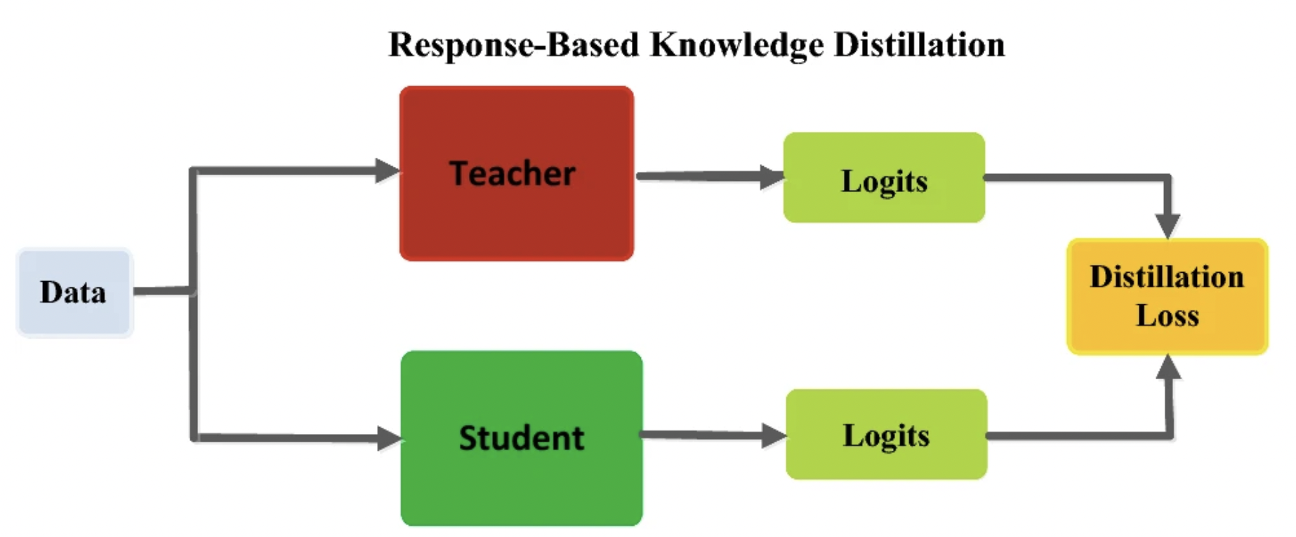
Other distillation approaches—such as feature-based KD, relation-based KD, and the contrastive approach described above—do exist, but require more intimate knowledge of the teacher’s features and/or layers
Methods and Experiments
We center our studies on a standard dataset of 10k English words scraped from high-level Standard English texts that’s been empirically validated for quality. We also use the OpenAI API to obtain text-embedding-ada-002 embeddings of the entire dataset to use as ground truth. While these aren’t necessarily the best embeddings, even among OpenAI’s own embeddings, they are the best choice given our computational restrictions.
Now, we detail our model architecture. Our baseline model (call this Model A) is a sequential ReLU and nn.Embedding layer followed by L2 normalization. Model A serves as a crude baseline—therefore, we do not investigate it as deeply as the more complex model that followed due to large differences in performance.
Instead, we focus our efforts on the more complex Model B, detailed below in Figure 1 in the context of our pipeline. Model B utilizes an nn.Embedding layer, followed sequentially by 2 blocks. The first uses ReLU activation followed by a linear layer of size \(\frac{\text{embedding_dim}}{2}\). The second layer is the same, except the final Linear layer outputs embeddings with the full “embedding_dim.” Notably, we use L2 normalization to make sure each embedding vector has magnitude 1 (such that all embeddings exist in an n-hypersphere.) Since all embeddings are unit embeddings, using cosine embedding loss along an Adam optimizer is natural. Thus, instead of computing cosine similarities between teacher and student vectors, we can just focus on minimizing this embedding loss.
For the training stage, we train our embedding model to map words to vector embeddings on Google Colab with an Nvidia T4 GPU. There may be up to 3 processing steps, as depicted in Figure 1:
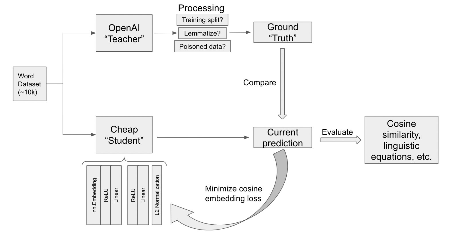
First, we choose whether or not to lemmatize the entire dataset before proceeding.
Second, the training split. We train our embedding models above on each of the following proportions (call this \(p\)) of the dataset: 0.005, 0.009, 0.016, 0.029, 0.053, 0.095, 0.171, 0.308, 0.555, and 1.00.
Finally, we choose whether or not to poison 10 percent of the entire word dataset (not the training dataset). When a word is poisoned, the model incorrectly believes that some random unit vector is the ground-truth embedding instead of the actual OpenAI embedding.
For each such model, we train for up to 80 epochs, limited by our computational resources.
We then evaluate the model’s embeddings against the ground truth with multiple metrics—cosine similarity (via the embedded cosine loss), graphically via distributions of the embedding means, linguistic math, etc.
Taken together, this methodology is comprehensive.
Results and Analysis
Model A, the Baseline
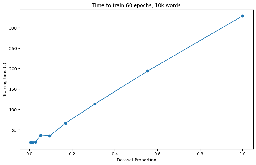
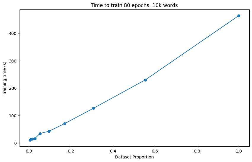
First, here is a graph of training up our baseline Model A (Figure 2) and our augmented Model B (Figure 3). The difference in epochs (80 for Model A, and 60 for Model B) training is due to limited resources. This doesn’t matter much, as a clear, near-linear relationship between \(p\) and training time, which we use to estimate used computational resources. Thus, we consider \(p\) as inversely proportional to the computational resources used for all our experiments.
For Model A (with no lemmatization, no data poisoning), we also want to visualize the tradeoffs between the number of epochs trained, the training proportion \(p\), and the training loss to establish some baseline intuition. To this end, we take inspiration from the game theoretic concept of Pareto efficiency, which aims to find equilibria where no change improves one of these 3 factors without hurting one of the other 2.
We also wanted to visualize the tradeoffs between the number of epochs trained, the training proportion, and the cosine embedding loss, since we are motivated to find the optimal balance of these 3 factors. See Fig. 4.
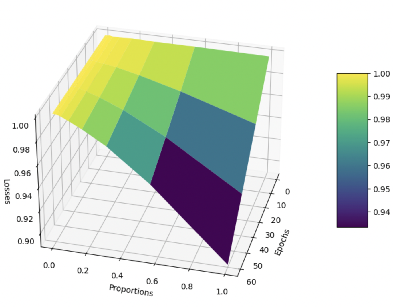
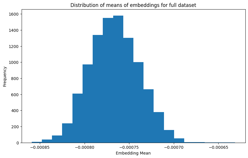
Unfortunately, Fig. 4 is not particularly enlightening. Training loss decreases as the number of epochs increases and as training proportion \(p\) increases. There are also no local minima or maxima of interest. Figures 5 and 6 also confirm this with their plots of distributions of embedding means. Specifically, as we tend to move towards the right and bottom of Fig. 6, i.e. we train longer and on more data, we simply seem to approach the true distribution (Fig. 5) without anything of note.
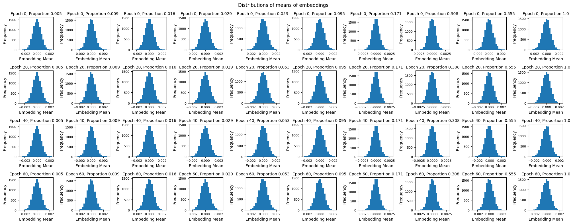
These results motivate us to look beyond our Model A. Our results from this point focus on Model B because we didn’t want a poorly performing model like Model A to be a true control, it merely served as an intuitive baseline.
Model B, the Baseline
As in the previous part, we obtain a Pareto-like graph for Model B, without any lemmatization and data poisoning. Firstly, the cosine embedding losses are much lower than before, due to the improved model architecture. More interestingly, after about 10 iterations, the training loss seems to stabilize across all versions of the model, potentially suggesting that training longer may not be worthwhile.
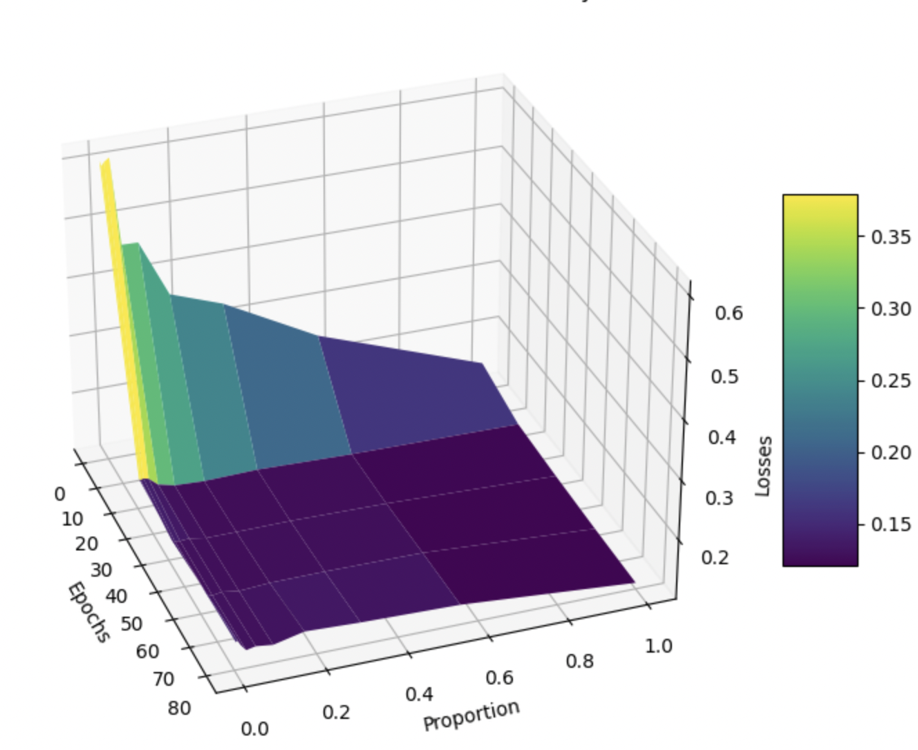
Since this is our base model, we don’t investigate further.
Model B, Lemmatization, No Poisoned Data
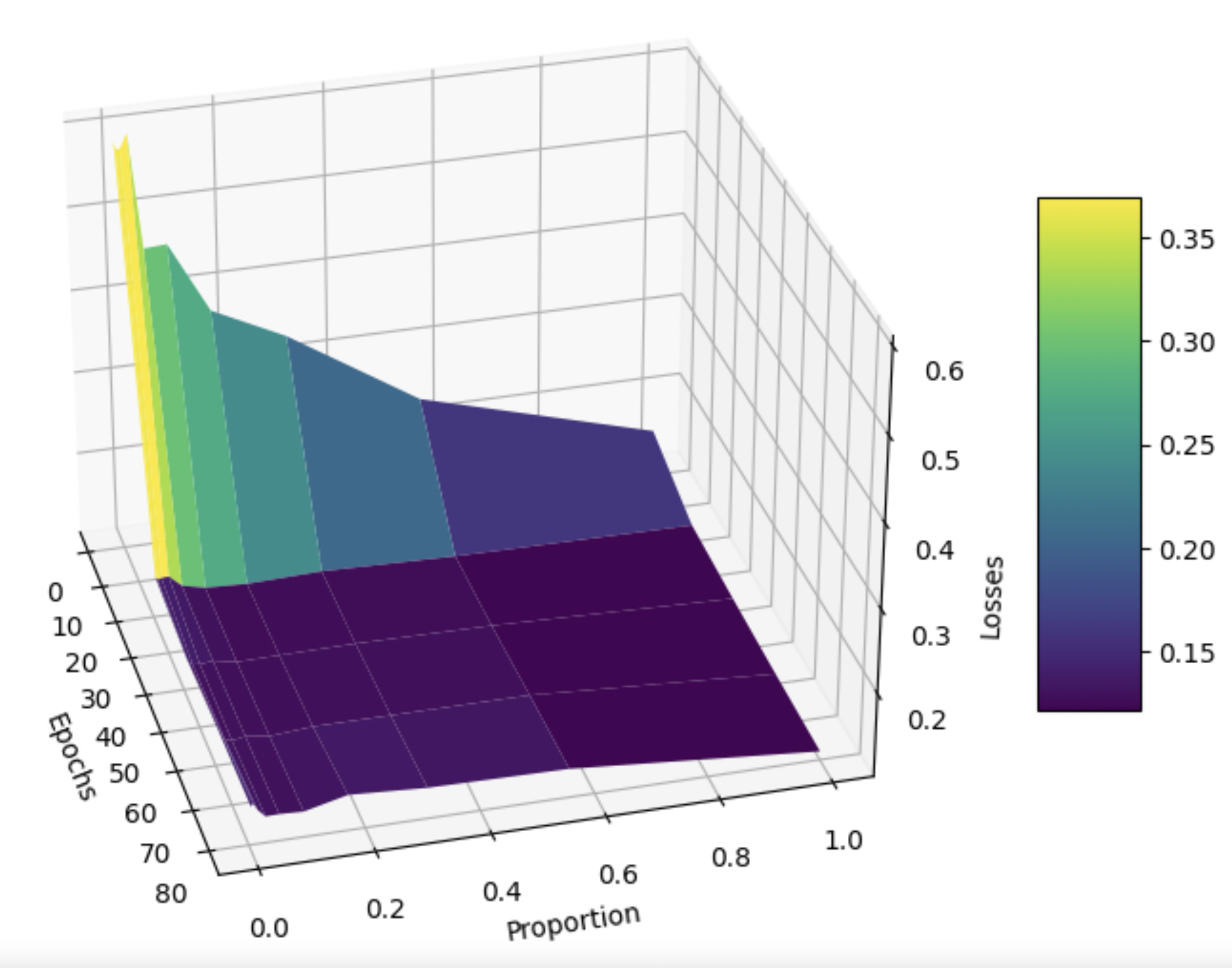
Now, we look to Model B, with lemmatization, but no poisoned data. The Pareto-like curve for this is telling (Fig. 8), with it looking very similar to the baseline Model B’s. As before, this suggests that training for longer may not be worthwhile, and could potentially lead to overfitting.
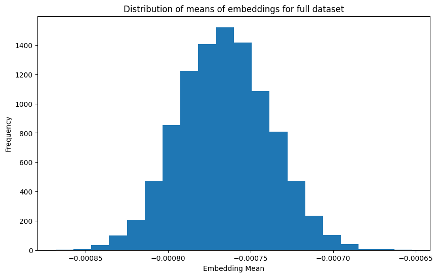
We also have a distribution of the means of embeddings for the whole dataset (Fig. 9) and from each variant of the model at different epochs (Fig. 10). Again, the results don’t say anything surprising: as we train on more data for longer, the distribution approaches that of the training dataset.

To check for overfitting, we will later validate our model on simple linguistic tests, as described in the very beginning. Specifically, we will validate our model’s performance on linguistic math against OpenAI’s performance.
Model B, Lemmatization, Poisoned Data
The following is the Pareto-like curve, except now we poison 10 percent of the entire dataset, as described in Methods/Experiments. Curiously, we find a local minima at approximately \(p = 0.1\) and ~20 epochs, demonstrating that our overall approach of training on a small fraction of the dataset naturally resists moderate-scale adversarial attacks on our ground-truth embeddings. Of course, the addition of poisoned data means that the loss values are on average higher than those in the previous subsection, where there was no poisoned data.
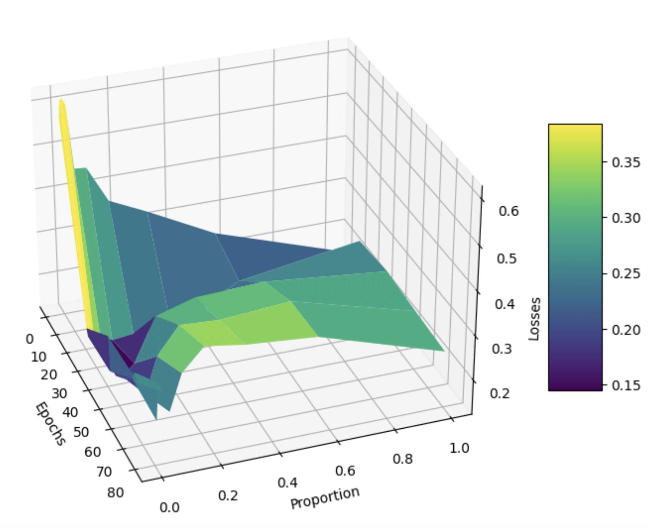
Again, looking at the distribution of the means of embeddings (see below), we see that models that trained on too much of the data are completely ruined. We don’t even need to compare these distributions against the whole-model distribution to see this. This result demonstrates that even a relatively small amount of poisoned data can manipulate a naive embedding model trained on an entire dataset.

The Effects of Data Poisoning and Surprising Robustness
As discussed previously, we want to externally validate our models with both linguistic equations and pairs of synonyms. Essentially, we want to check that our student groups together similar words like the OpenAI teacher. Since our poisoned model performed best with \(p = 0.095,\) we use this training proportion to compare Model B with lemmatization, but no poisoned data to Model B with lemmatization and poisoned data.
For clarity’s sake, we focus on single a representative example of our validation results in this blog. Specifically, we look into “nonviolent” and “antiaggressive,” which intuitively should exist close together in the n-dimensional unit hypersphere. Using dimensionality reduction techniques to visualize this in 2D, we obtain the following:
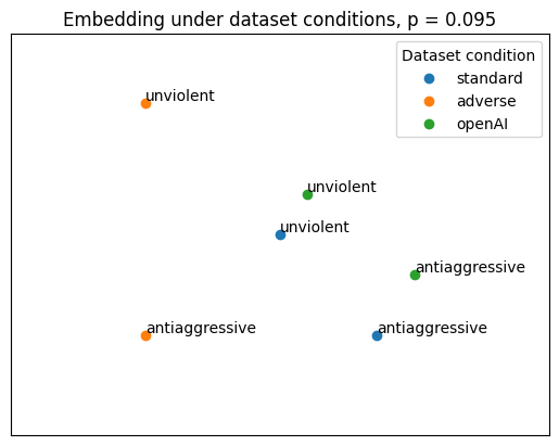
The poisoned model is surprisingly performant, performing decently against both the unpoisoned model and the OpenAI model. These results support our notion that student models that train on as little of the data as possible are somewhat resistant to uniform, random adversarial data poisoning. This empirical result is encouraging, especially since our data poisoning threshold was somewhat high.
Conclusion, Discussions, and Future Directions
On balance, our results help us answer our question about how to best mimic OpenAI’s word embeddings without excessive API calls. We utilize a spin-off of a response-based KD architecture to train our student model under different conditions, demonstrating both that certain preprocessing (lemmatization) improves our embedding model and that training on smaller amounts of data creates more robust models that resist adversarial data. Our initial results demonstrate promise and serve as a call to action for others to research other cheap, robust word embedding models.
To be clear, there are certainly many limitations to our study. For one, we keep our modeling architecture simpler due to our limited compute, while a real model would certainly use a different architecture altogether. Our dataset was also on the smaller side and doesn’t fully represent the English language. Also, our implicit use of time as a proxy for computation (especially on the erratic Google Colab) is imperfect. Also, preprocessing (including, but not limited to, lemmatization) may require substantial computational resources in some cases, which we don’t account for.
Additionally, many of the constants that we chose (such as the 10 percent data poisoning threshold, the proportions of data we trained on, etc.) are arbitrarily chosen due to limited compute. This could’ve caused unexpected issues. For example, the output dimension of embedding Model B, 1536, is more than 10 percent the size of the dataset (10k). Thus, due to our relative lack of data, our trials with data poisoning can encourage non-generalizable memorization, which is not ideal.
Future directions would include exploring other types of preprocessing, as hinted at in our literature review. We could also look into different types of adversaries—perhaps smarter ones that actively feed information that they know to be detrimental to the model, instead of some random unit vector. While we didn’t have robust supercomputer access, we’d also love to be able to test out fancier embedding architectures.
Finally, we’d like to thank the 6.S898 faculty and TAs for their support!