Examining assumptions in scRNA-seq foundation model pre-training (6.S898 Final Project)
Final project for MIT's Deep Learning (6.S898) class.
Introduction
If the fundamental building block of biology is the cell, then the fundamental building block of cells are genes. Genes are small segments of DNA that encode the information to create a protein, and proteins are a diverse set of macromolecules that can perform a staggering range of chemical functions which, when taken all together, lead to the complex behavior of cells and the organisms they make up. To create proteins from genes, an intermediate “data transfer” occurs through another molecule type known as RNA. This information flow of genes to RNA to proteins is typically referred to as “gene expression”, and is so core to biology that it’s also known as the “central dogma of molecular biology”.
Due to the importance of gene expression, many technologies have been developed to make quantitative measurements of gene expression from cells. One of the most prominent technologies is called single-cell RNA sequencing (scRNA-seq), which enables the measurement of the expression of all genes in a given cell, often measured across thousands of cells simultaneously
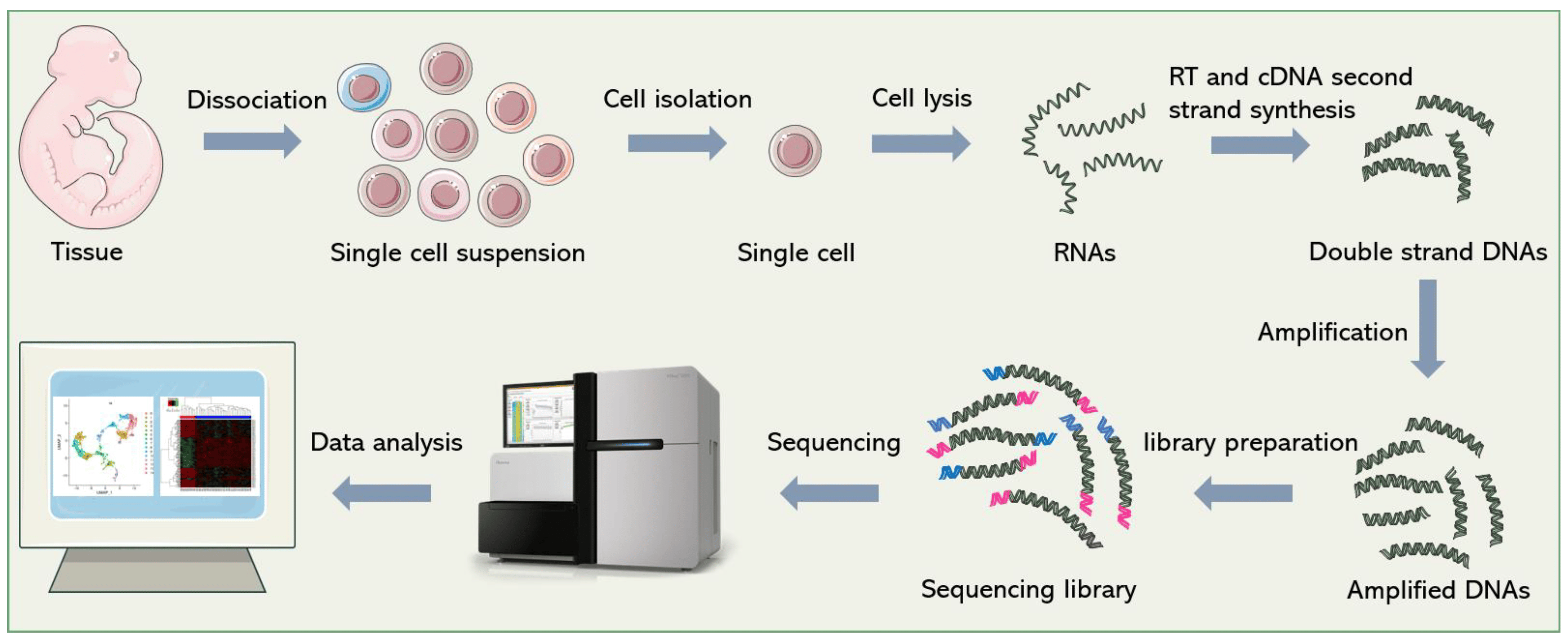
Large scale scRNA-seq datasets have enabled the high-resolution profiling of different organs and tissues at the cellular level, uncovering diverse cell types, rare subpopulations, and dynamic gene expression patterns within complex tissues and organisms. This technology has found applications in various fields, from developmental biology and immunology to cancer research and regenerative medicine.
While scRNA-seq has seen broad-scale adoption, many challenges remain. In particular, an individual research experiment may focus on a particular cell or tissue type, and produce insufficient data to apply modern machine learning techniques. To supplement their data or to gain additional context, a researcher may wish to utilize data generated from other experiments or researchers. However, performing large-scale integration of datasets across samples, tissues, and experiments currently presents challenges of scalability and non-biological differences between datasets driven by experimental variability (colloquially referred to as “batch effects”)
In parallel to the explosion of available scRNA-seq data, the machine learning field has seen an increasing trend towards “foundation models”. Foundation models are large-scale deep learning models pre-trained with vast amounts of data for the purposes of creating a generalizable representation of a particular datatype (e.g. text, images). Given these developments, recent work has focused on developing scRNA-seq foundation models as an approach to solve the challenge of integrating diverse sets of scRNA-seq datasets in a scalable and generalizable way
In this post, we’ll explore a fundamental assumption of three such models (Geneformer
What exactly is a rank-value encoding? Well, a typical representation of gene expression is a vector \(x \in \mathbb{R}^N\), where \(N\) is the number of genes, and each entry is a measure of the corresponding gene’s expression. In a rank-value encoding, gene expression is instead represented as a list of N strings, where the strings are gene names, and are ordered in descending order of the underlying gene expression value.
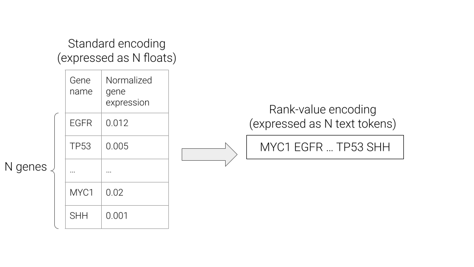
The rank-value encoding provides an intuitive transformation of the continuous gene expression values into an English language sentence that is compatible with existing approaches for foundation models in the natural language processing (NLP) field. However, as can be seen above, the rank-value encoding also drops the information of the exact gene expression values. Hopefully by the end of this post, we’ll have gained some intuition for how a rank-value encoding of gene expression could be hindering the development of foundation models for gene expression and see that this does play out in practice for a real scRNA-seq foundation model.
Related work
Overview of gene expression representations in foundation models
While we won’t go into a full detailed comparison of different methods for constructing gene expression foundation models from scRNA-seq data, it’s worth spending a little time discussing the commonalities and differences of various approaches at a high-level.
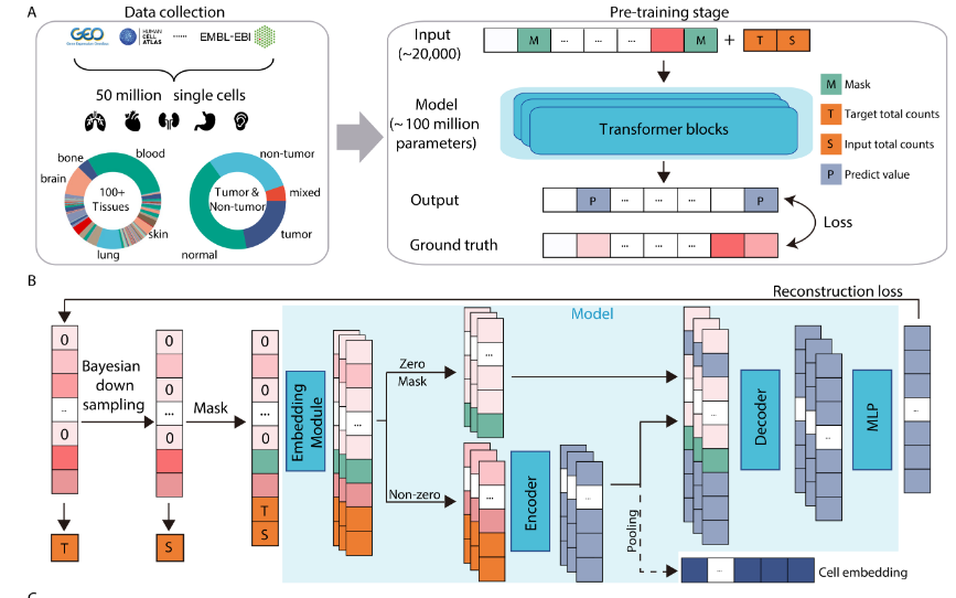
The most important distinction for this post is between methods that use a rank-value encoding and those that don’t. For methods that don’t use a rank-value encoding, we see a further distinction between methods that employ some form of value-binning, where continuous expression values are mapped to a discrete number of pre-specified bins, and those that don’t. Methods that use a binning approach are scGPT
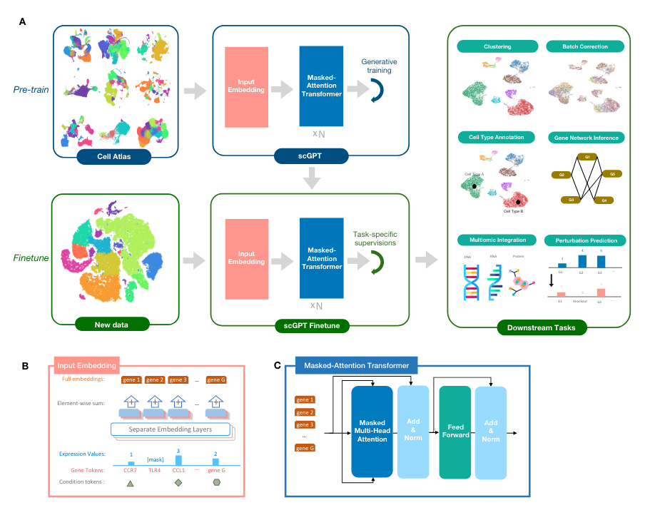
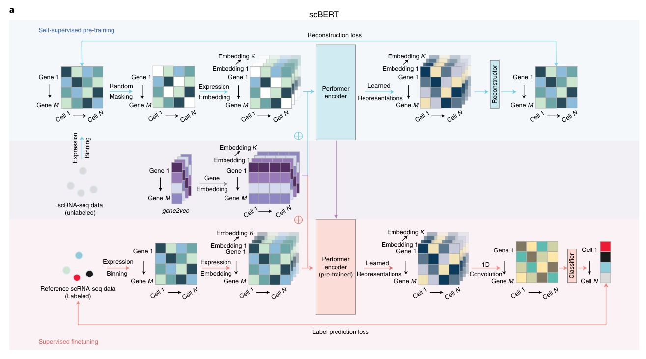
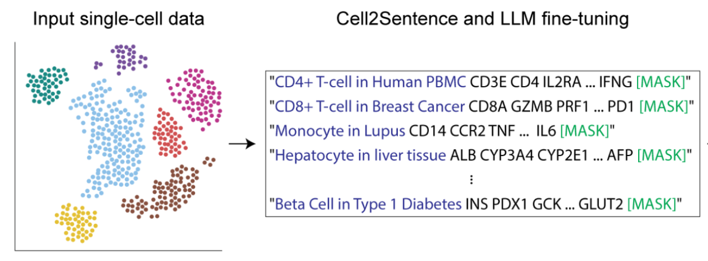
On the other hand, we have the methods that we’re most interested in for the purposes of this post: the ones that utilize a rank-value encoding of gene expression. These methods are: Geneformer


Critical examinations of scRNA-seq foundation models
In light of the recent development of many approaches for scRNA-seq foundation models, researchers have also begun performing critical assessments of such models. One of the main value propositions of foundation models is generalization to new data in a few-shot or zero-shot manner. To test this hypothesis, Kedzierska et al.
However, both of the works discussed above focused on examining the performance of scRNA-seq foundation models as a black box, whereas to the best of our knowledge, there are no current works examining the fundamental assumptions implicit in these foundation model approaches. We hope to begin addressing that gap in this post. By understanding whether or not rank-value encoding well-approximates the real similarities and differences in gene expression across cell types, we hope to either validate this assumption or gain insight into future avenues for improving pretraining of such scRNA-seq foundation models.
Methods
Dataset
To perform our assessment of rank-value encoding, we’ll work with the Tabula Sapiens dataset
We use the final dataset from Tabula Sapiens, which has already been subjected to quality control assessment, filtering, and normalization. While we won’t go into the details of their pipeline here, these are available in their manuscript for the interested reader. In line with typical scRNA-seq workflows, we also subset the full set of ~22,000 genes down to a subset of 2,435 genes that have been marked as “highly variable genes” (HVGs) in the Tabula Sapiens dataset. This is a fairly standard step in scRNA-seq data processing workflows, as many genes are constitutively expressed across cell types, and thus provide little information for distinguishing between cell types. Highly variable gene selection was performed by the Tabula Sapiens Consortium following the methods and recommendations in Seurat

Additionally, since the Tabula Sapiens dataset is quite large and also has some cell types that are disproportionately represented, as shown above, we’ll also subset the data to get a more tractable dataset for experimentation. To do so, we’ll focus on cell types with 500 or more examples, and then further randomly subsample to 500 cells per type. This leaves us with 89 cell types
To interact with this data, we’ll be using the AnnDatascanpy
Assessments
To assess how well a cellular state can be represented using a rank-value encoding of genes, we’ll look at various measures of similarity in the raw gene expression space and the rank-value encoded space, and compare those measures both within cell types and between cell types. We’ll calculate the following measures for all pairs of cells:
- Euclidean distance of UMAP-projected gene expression values
- Spearman rank correlation coefficient
- Euclidean distance of UMAP-projected Geneformer embeddings
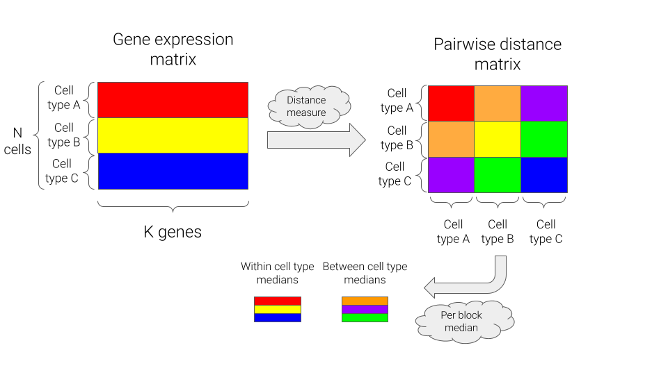
For each distance measure, we can then generate comparisons at the level of cell types by summarizing via the median of the pairwise distances, either within or between cell types. A schematic of this approach is shown below.
UMAP of gene expression values
The idea behind this comparison is to utilize the continuous gene expression vectors, but using UMAP (Uniform Manifold Approximation and Projectionumap-learn Python package with defaut settings and n_components=5. Once we have the per-cell projections, we calculate Euclidean distance between all pairs of cells.
Spearman rank correlation coefficients
The Spearman rank correlation is a non-parametric measure of correlation between two ranked lists, which we can leverage to obtain a direct comparison of rank-value encoded gene lists. To accomplish this, we first calculate a rank-encoding of each cell’s gene expression, with identical values being assigned a fractional rank equal to the mean of their ordinal ranks. As the Spearman correlation is defined as the Pearson correlation on the rank-encoded lists, we can then directly calculate the Spearman correlations between all pairs of cells.
Euclidean distance of UMAP-projected Geneformer embeddings
To fully assess the effect of rank-value encoding in a deep learning model, we take this one step further by calculating the embeddings of our cells using Geneformer. We generate these embeddings by using their model and code as hosted on HuggingFace for tokenization and embedding of our gene expression vectors. For each cell \(i\), we obtain an embedding vector \(x_i \in \mathbb{R}^{256}\). We further project these 256-dimensional vectors down to 5 dimensions using UMAP for consistency with the projections of the raw gene expression values described above, and then calculate Euclidean distance between all pairs of cells. The rationale here is that Euclidean distance between two points may be larger in a 256-dimensional space than a 5-dimensional space due the high dimensionality (i.e. “curse of dimensionality”). However, we do still see similar results when using the full 256-dimensional embedding vectors (see Appendix).
Results
Rank-value encodings preserve similarity between cell types
The first thing we can see from our results is that rank-value encodings do preserve similarity between cell types in a similar manner as distances generated from raw gene expression values. The figure below is generated by looking at the distributions of distances between pairs of cells from the same type (“within”) or from different cell types (“between”). To provide a comparison at the level of cell types, we plot the median of each distribution rather than individual pairs of cells, i.e. the “within” group contains 89 data points and the “between” group contains \(\frac{89 \times 88}{2}\) data points.

How should we interpret this? What we can observe is that all three measures maintain high similarity for cells from the same type and less similarity for cells from different types. Put another way, rank-value encodings do define a space in which different cell types tend to be distant and cells from the same type tend to be near each other. We can also say that this holds when using both a non-parametric measure of the rank-value encodings (Spearman rank-correlation) and also when using a deep learning model that operates on rank-value encoded gene vectors (Geneformer).
However, we do also see that the difference between the “within” and “between” cell type distances is more pronounced when using a non-linear function on the raw data compared to either of the methods operating on the rank-value encoded gene vectors. This difference will become even more clear as we look at joint distributions of our different measures in the next section.
Raw gene expression values better preserve within cell type similarities
To gain further insight into how rank-value encodings compare to raw gene expression values, we can look at the joint distributions of our distance measures. Below we see the joint distribution of our raw gene expression-based distances compared to the rank-correlation values, shown as a 2D histogram where each hex is colored according to the number of points that fall within that bin.
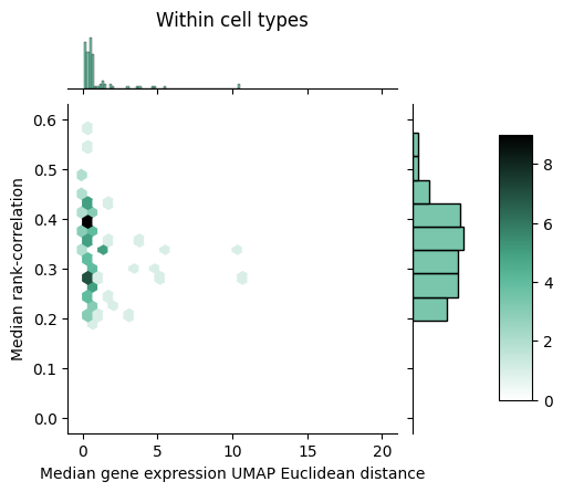
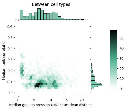
We can notice that within cell types, the rank correlation has a fairly wide dynamic range whereas the raw gene expression-based distance seems to show a tighter packing. Between cell types, we can observe that the rank correlations largely clump up closer to zero but do mesh with the larger distances we see with the raw gene expression-based measure.
Given that we see a spreading out of cells within a type using a rank correlation, the natural question becomes whether this holds when we use a deep learning model that can learn a complex non-linear function of the rank encodings. That’s exactly what we look at below where we perform a similar comparison, but swapping out the rank correlation distance measure for the distance measure based on Geneformer embeddings.

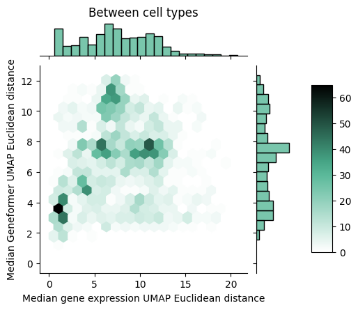
With the Geneformer embeddings derived from the rank-value encodings, we now see that the between cell type distances are better matched to the distances derived from raw gene expression values. However, we still see that Geneformer embeddings are more spread out within cell types compared to the non-linear transform of the raw gene expression values. To better understand why this might be the case, we propose one possible contributing factor in the next section.
Sparsity of scRNA-seq data may drive loss of information in rank-value encodings
A key aspect of scRNA-seq data is its extremely high sparsity. When working with single cells, the amount of available RNA is already quite limited, and then each processing step, such as RNA isolation or sequencing, introduces technical noise and the possibility of “dropout events”, where a gene’s expression is not detected at all. Combined with the inherent stochasticity of gene expression, we’re often left with data where the vast majority of genes have zero detected RNA molecules.
Shown below is a histogram of sparsity per cell in the full Tabula Sapiens dataset as well as in the subset of cells and genes we considered in the analyses above.
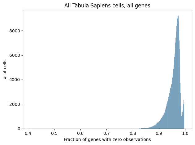

While many methods for processing scRNA-seq data attempt to handle the high sparsity in a principled manner, most of the methods described here simply remove genes with zero observations from consideration. In particular, scGPT, GenePT, and Geneformer all remove genes with zero observations from their inputs, and cell2sentence restricts itself to the 100 genes with the highest expression per cell, effectively removing all genes with zero observations. While sparsity is at least partially driven by stochastic technical factors, there is undoubtedly a biological contribution as well, which may be removed when dropping genes with zero observations. While this issue is not unique to rank-value encoding, we can see that all of the methods we’ve discussed here that use rank-value encoding remove genes with zero observations, likely to circumvent the ambiguity in how one would enforce an ordering on genes that all have zero observations.
Discussion
To give a high-level summary, what we’ve seen in this post is that rank-value encodings are an appealing way to transform continuous gene expression vectors into a format that’s directly compatible with the foundation model architectures that have seen great success in natural language processing. However, they also seem to lose some valuable biologlical information of cell types, particularly information concerning similarity of cells within a given type.
While we don’t present a smoking gun for an exact characteristic of this loss of information, we present sparsity as a key challenge in scRNA-seq data, which may be exacerbated when using rank-value encodings. We can also further hypothesize that rank-value encodings may be sensitive to small changes in gene expression values from technical noise, which could cause a shifting of ranks and thus amplify the impact of said noise. Similarly, rank-value encodings lose the absolute quantification of gene expression, and this loss of granularity may impact the model’s ability to capture the cases where subtle differences in gene expression hold biological significance.
From the perspective of downstream use cases, models based on rank-value encodings are also limited in their ability to explore the counterfactuals that may be interesting in cases such as predicting cellular responses to a novel therapeutic. For example, if a drug were known to affect the expression of a single gene, but not to the point where the ranking of this gene shifted, then such a model would be unable to explore the downstream effect of this drug on the expression of other genes.
In terms of limitations, the work presented here is fairly superficial and is constrained both in terms of size of datasets and breadth of methods compared. To perform a more robust comparison in the future, we would like to scale up this analysis to larger datasets, such as the full Tabula Sapiens dataset. We would also like to more directly compare cell type similarities in the embedding spaces of other scRNA-seq foundation models, including those that do and do not utilize rank-value encodings. A great follow-up would be to perform a head-to-head comparison of a model like scBERT to Geneformer on the full Tabula Sapiens dataset.
Additionally, we’ve also yet to explore the angle of robustness across datasets. It’s possible that some of the shortcomings we’ve listed for rank-value encodings may actually be benefits in the context of supppressing technical noise when integrating scRNA-seq datasets across studies, institutions, and experimental techniques. Performing this comparison across datasets would be a valuable follow-up that would help paint a more full picture of the value of rank-value encodings in the context of constructing foundation models for gene expression data.
While we’ve discussed many challenges in constructing foundation-scale models for gene expression data, it’s worth closing this post with an optimistic reflection on the potential value of such models. By training a deep learning model to construct a representation space of cellular state, we stand to create a powerful tool that will help us gain a fundamental understanding of cellular biology and its underlying complex regulatory networks. Ultimately, such tools could help us unravel the genetics of various diseases, paving the way for a new era of disease treatments and precision medicine.
Appendix

