Leveraging Representation Engineering For LLM’s In-Context-Learning
We present a method to observe model internals whether LLMs are performing in-context learning and control the model outputs based on such Context Vectors.
Introduction
Emerging capabilities in deep neural networks are not well understood, one of which is the concept of “in-context learning” (ICL), a phenomenon where the a Large Language Model (LLM)’s understanding of the prompt and ability to answer accordingly drastically increases after being shown some examples that answer the question. Evaluating in-context learning and understanding why the behavior happens is both an interesting theoretical research question and a practical question that informs directions to conduct research that further advances LLM capabilities by, say, exploiting more of in-context learning.
We attempt to explore the phenomenon of in-context learning by leveraging another exciting field of work on mechanistic interpretability where researchers set out to understand model behaviors by interpreting and editing internal weights in models. One such work that we base on is Representation Engineering by Zou et al. (2023)
We propose to use methods in Zou et al. (2023)
We then explore the results of controlling the activations along the “Context Vector” direction, in the hope that editing the activitions would further boost the performance on top of in-context learning. We compare the model outputs on the classification datasets in a zero-shot setting and a setting of natural in-context learning, with the “Context Vector” amplified, and suppressed. While we find boosting performance through such editing to be challenging and sometimes finicky to tune, we find the results to be promising on editing weights to suppress the context that the model draws from and drastically reducing the performance.
Background & Related Work
In-Context Learning (ICL)
An LLM is frequently aseked to perform a task in inference time that many realized providing some examples of how to answer the task can drastically improve the model’s performance. This phenomenon is called in-context learning. For example, Zhou et al. (2022)
In other scenarios, the LLM does not need to rely on prompts at all and can deduce the pattern from the few-shot examples alone to predict the answer. While there is no universal definition of in-context learning and its meaning has shifted over time, we define it as the performance boost to answer questions based on a limited amount of examples (as the context).
Interesting, Min et al. (2022)
Theories on why ICL happens
While the concept of ICL is well studied, the underlying mechanism of ICL is not well understood. Xie et al. (2022)
Akyürek et al. (2022)
Furthermore, Olsson et al. (2022)
While many hypotheses and theories have been proposed to explain ICL, most explorations to prove their theory has been small in scale, and the literature lacks a study on the large-scale LMs’ internals when performing ICL.
Model Editing & Representation Engineering
We’ll use the Representation reading and controls methods presented in Zou et al. (2023) to understand the context where the model attends to and discover directions that indicate such reasoning.
Relatedly, there have been a recent surge in research related to model knowledge editing, including Meng et al. (2023)
Experiment Setup
Datasets
We adopt a total of 30 datasets on binary classification, (sentiment analysis, natural language inference, true/false inference) and multiple choices; 16 datasets are used by Min et al. (2022) tweet_eval and ethos dataset families, rotten_tomatoes, and ade_corpus_v2-classification. Following Min et al. (2022)k=64 examples in the test for few-shot training, and the rest are used for testing.
Training Data Generation
For training, we construct a set of context pairs for each dataset, each context pairs containing the same examples but different instructions. The instructions are “Pay attention to the following examples” and “Ignore the following examples” respectively, in the hope that by stimulating two opposites and examining the difference, we can find a Context Vector that represents what the model draws from. We then truncate the example at each and every token till the last 5 tokens, so we can get a neural activation reading for each of the tokens.
A sample training data input using the rotten_tomatoes dataset is as follows:
[INST] Pay attention to the following examples: [/INST]
offers that rare combination of entertainment and education.
positive.
a sentimental mess that never rings true .
negative.
[INST] Ignore the following examples: [/INST]
offers that rare combination of entertainment and education.
positive.
a sentimental mess that never rings true .
negative.
Each context pair is identical except for the instructions. We use the context pairs to stimulate the model to learn the context and use the context vector to control the model’s behavior.
Testing Data Generation
For testing data, we use 3 input-labels pairs as the prompt, with the first two pairs serving as the in-context examples, and the last pair serving as the question that we actually want to test on, obfuscating the label from the prompt.
A sample testing data input using the rotten_tomatoes dataset is as follows:
Input:
[INST] offers that rare combination of entertainment and education. [/INST]
positive.
[INST] a sentimental mess that never rings true . [/INST]
negative.
an odd , haphazard , and inconsequential romantic comedy .
Label:
negative.
Model
We have explored using two models with 7 billion parameters, including Mistral-7B-Instruct-v0. and Llama-2-7b-hf; while we have found preliminary results consistent between the two models, all of our results later reported are from Mistral-7B-Instruct-v0 for consistency and due to a constraint on computational power and time.
Training Infrastructure
We used the MIT Supercloud infrastructure and a local machine with a single RTX 4090 GPU to train the model.
Results
We present results first on finding the Context Vector in the embedding space, then on using the Context Vector to control model outputs and evaluate their performance.
Representation Reading
We use the Representation Reading method presented in Zou et al. (2023) f$ and pairs of instructions $x_i$ and $y_i$, we denote the model’s response truncated at the $j$-th token as $f(x_i)_j$ and $f(y_i)_j$ and take the neuron activity at the last token of each of the responses, namely the activations of each and every token in the response.
We then perform PCA on the difference of the activations of the two instructions, namely $f(x_i)_j - f(y_i)_j$ and find the first principal component $v$ that maximizes the difference in the embedding space.
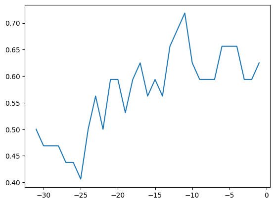
More surprisingly is the fact that we can find a clean representation of such Context Vector that correlates decently with the model inputs.
We use t-SNE to visualize the difference in the embedding space on the inputs of the 30 datasets across 32 different layers and report the results below.
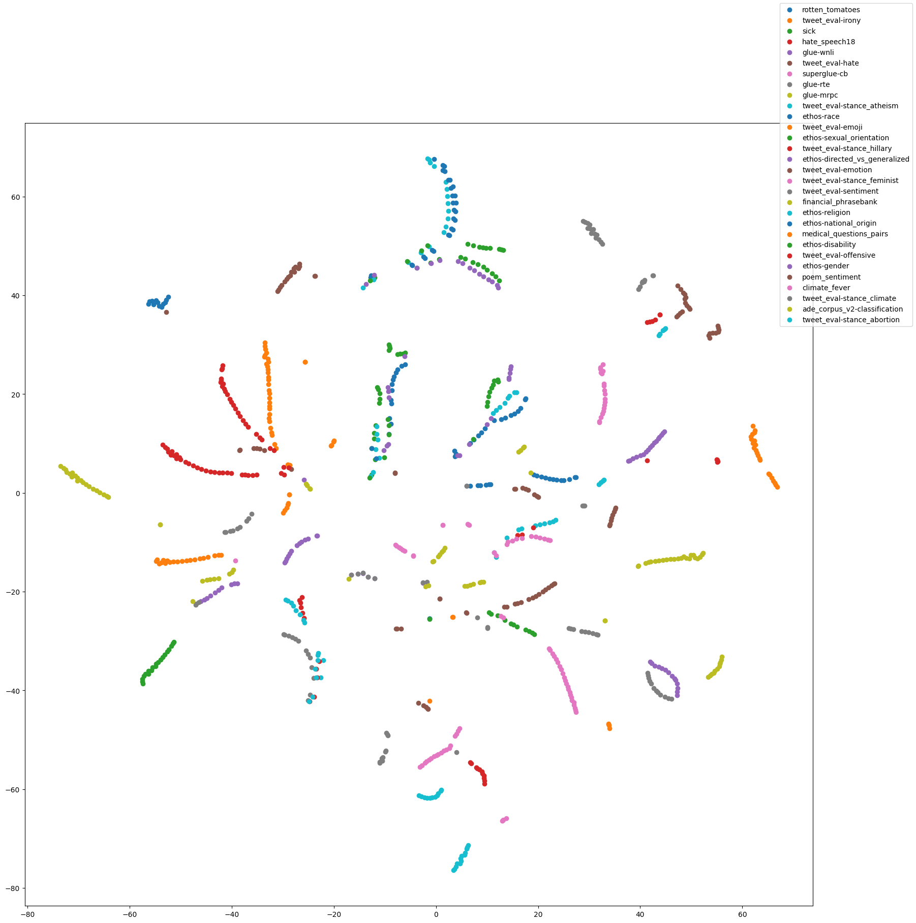
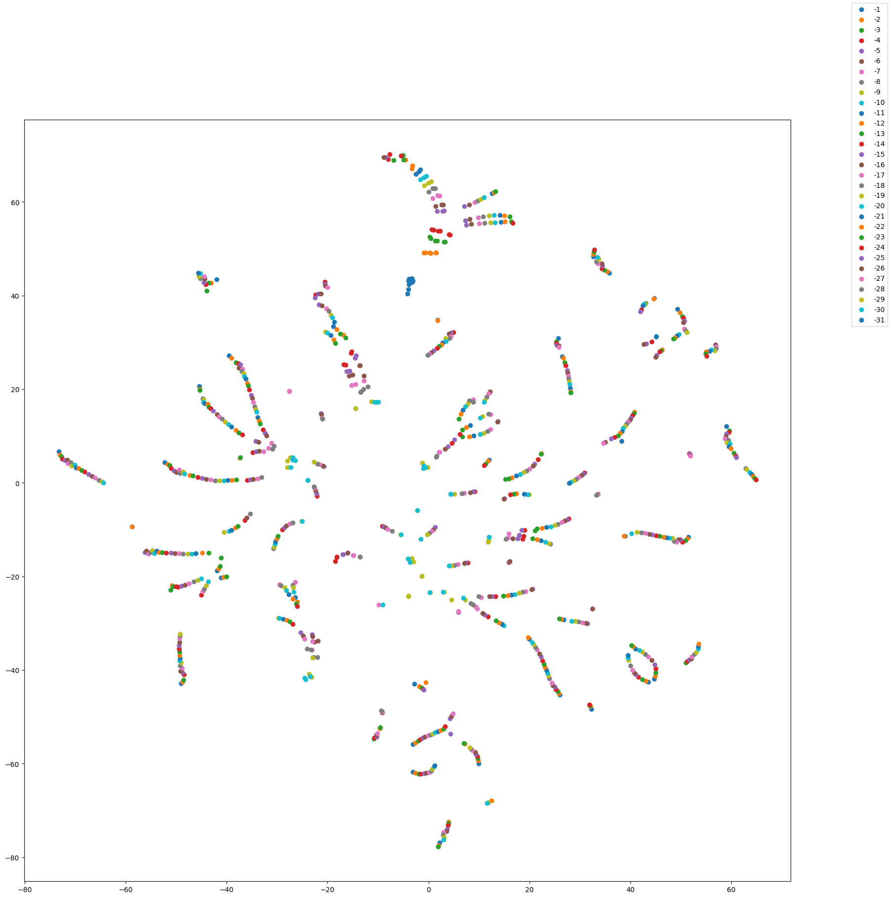
As shown in the figure, we find that the vectors are clustered by dataset, indicating that the Context Vectors are dataset-specific. There are no clear patterns across dataset or between different layers of the Context Vectors, further indicating that in-context learning activates different parts of the model’s latent space with information about different types of tasks.
We also conducted scans for neuron activities in the Context Vector across the different tokens of an example sequence in a similar style as Zou et al. (2023)
The following are the LAT scans for the neuron activities corresponding to a Context Vector trained on rotten_tomatoes sentiment analysis dataset evaluated on different dataset sequences. The following graphs further corroborate the findings above on the dataset-specificity of in-context learning; while the a sequence from the rotton_tomatoes dataset result in high neural activities for the Context Vector, most sequences from the other dataset do not, showing the uniqueness of such Context Vector. We have also observed most of the neuron activities in the later layers. This phenomenon makes sense since more abstract concepts and semantic structures formulate in later layers, thus being more correlated with the Context Vector, while earlier layers pick up more on token-level abstractions.
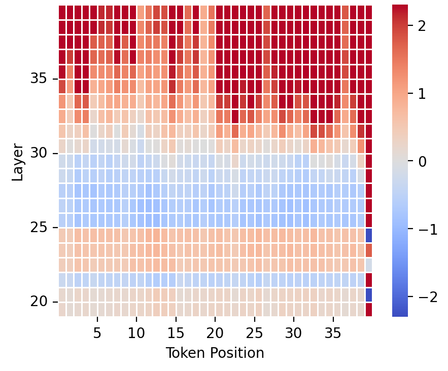
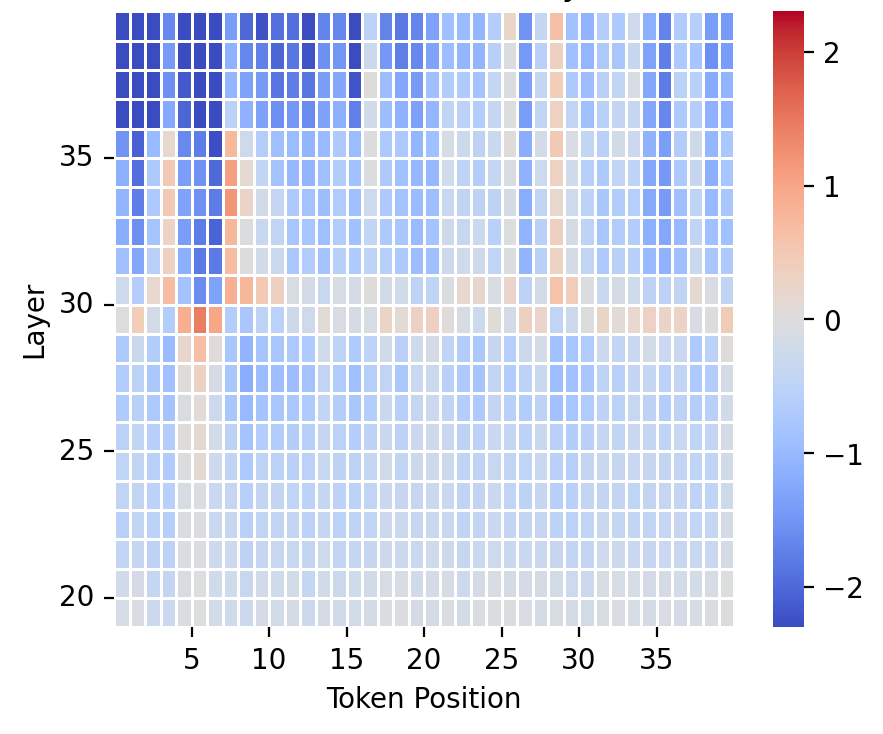
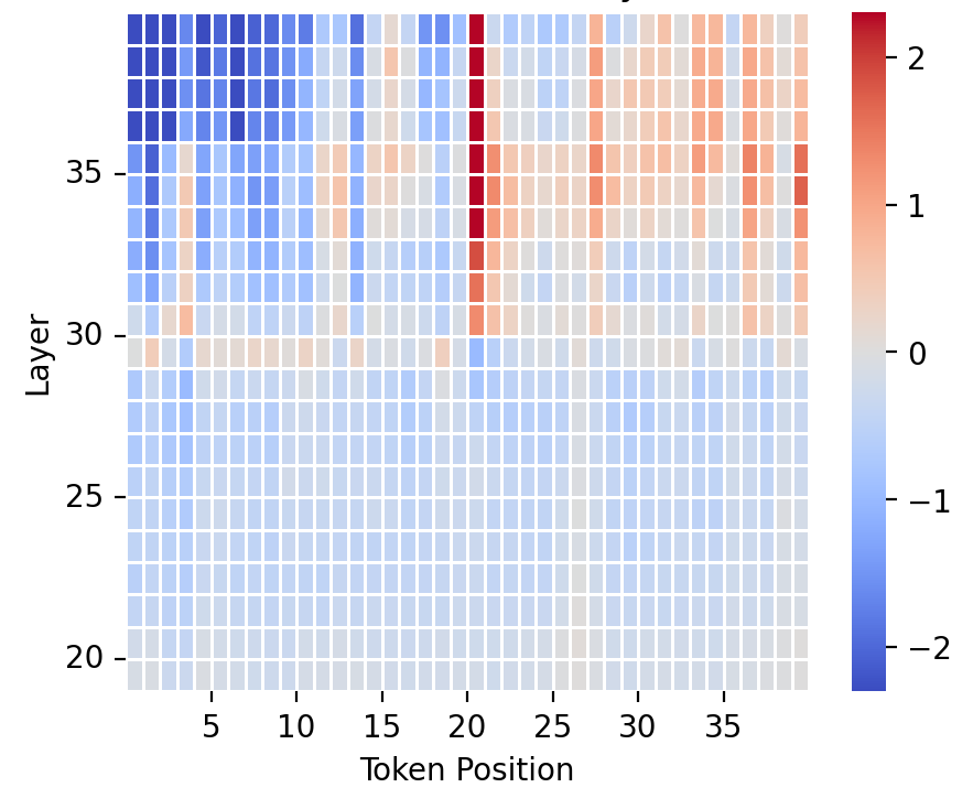
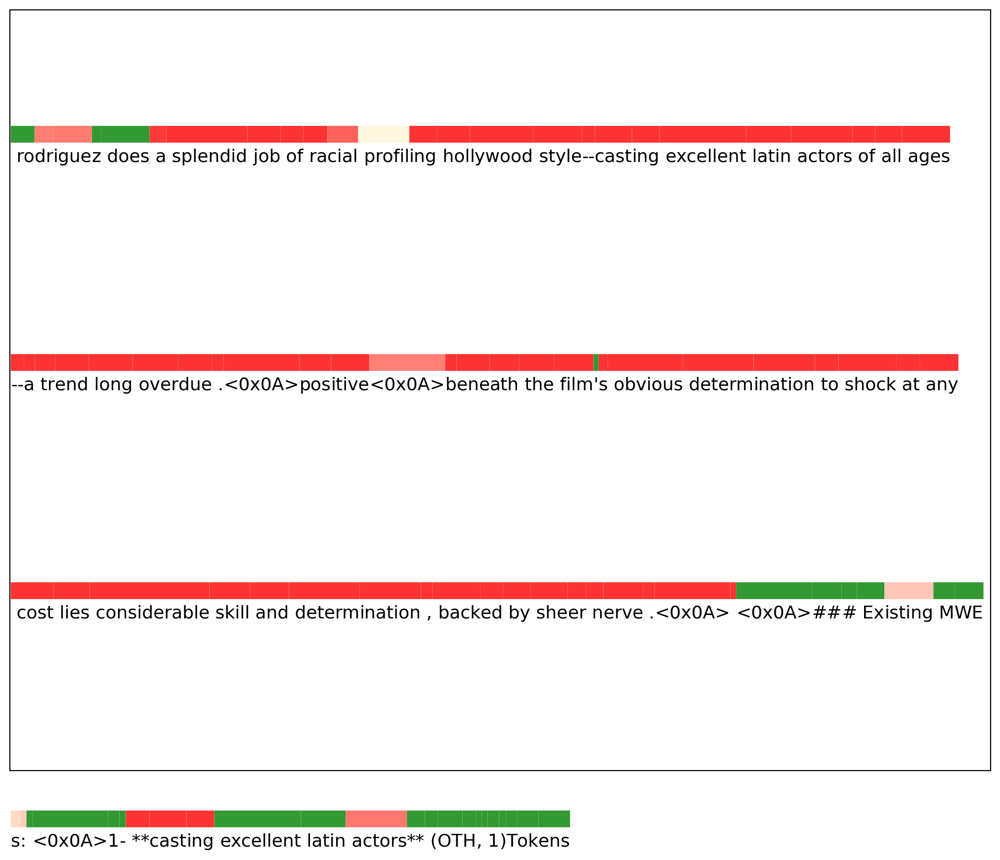
We have also produced graphs that zoom into the token-level neural activities detection on the Context Vector of the opposing pair (Pay attention & Don’t pay attention), shown below. A large difference in the neural activities of the two instructions is denoted by red and indicates that the ablation is effective, while the green shades indicate that there are similar in neural activities. The results show that the neural activities are consistently different across the sequence until the model starts generating next tokens and the context ends where the neural activities are similar.
Representation Control
To change an activation along some direction, we can imagine there are several canonical ways. First, given our Context Vector $v$ and an activation $a$, we can do one of the following.
Addition
\[a' = a + v\]Amplification
\[a' = a + \text{sign}(a \cdot v) v\]Projection
\[a' = a - (a \cdot v) \cdot \frac{v}{||v||^2}\]The first represents a constant perturbation so it supposedly transforms the representation to become more of a certain quality. The second amplifies the direction according to which side it is on, so it makes the representation more extreme. The third removes the quality from the representation by subtracting the projection.
We explore all these methods to control Mistral-7b-instruct. We do our experiments on the rotten_tomato, sick, hate_speech18, and glue-wnli in-context-learning datasets consisting of input-output pairings where outputs have two possible correct options – positive or negative contradiction or entailment, hate or noHate, and entailment or not_entailment (for sick, it originally contains a third option of neutral which we remove since our framework requires two classes).
Given learned representations with the same configuration as our representation reading, we construct a test set from the same dataset as training. The test set has $16$ examples, each with one demonstration followed by a question. We evaluate correctness by having the LLM generate $10$ tokens and checking if the correct answer is contained in the output and the incorrect answer is not contained in the output, without being sensitive to case. This ensures correct evaluation so that an answer of no_entailment does not evaluate as correct for having entailment inside of it if entailment is the right answer.
A hyperparameter which we denote $\alpha$ scales the size of $v$. If our Context Vector is $r$, sign value is $s$, then we have $v = \alpha \cdot r \cdot s$. We vary $\alpha \in { 0, 0.25, 0.5, 1, 2, 5, 10}$, and also take the negative of $\alpha$, which we label as positive and negative respectively.
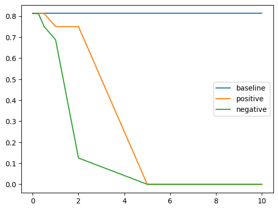
Results for Control with Addition
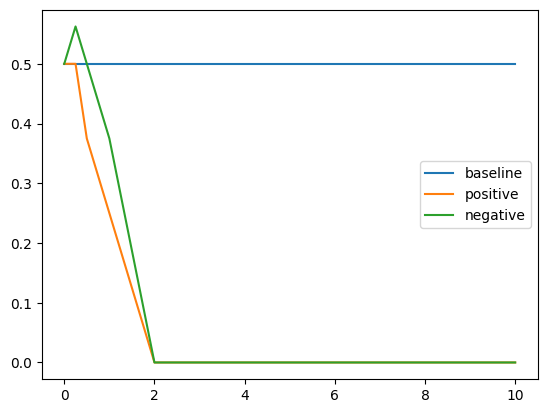
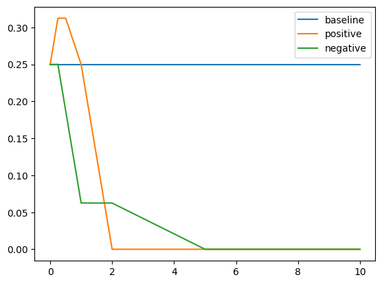
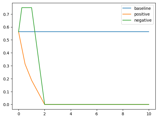
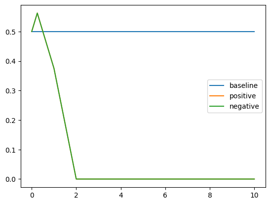
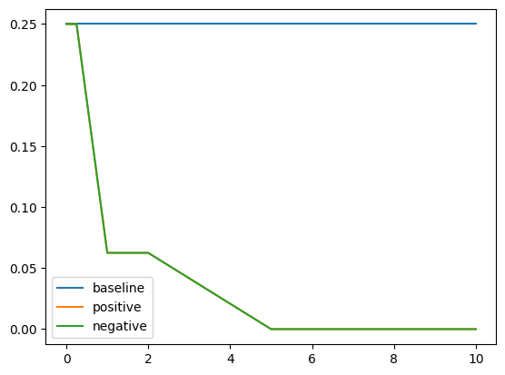
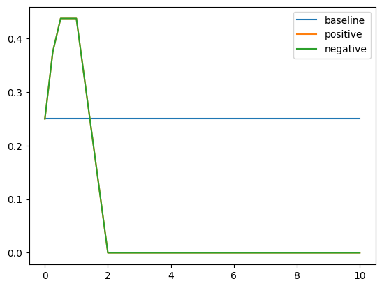
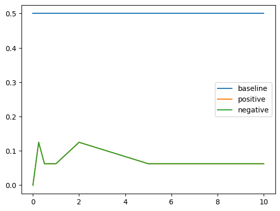
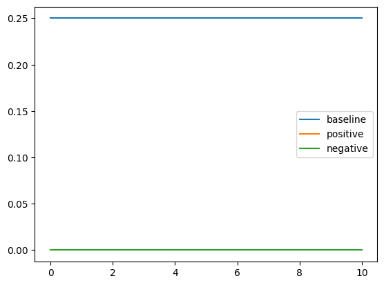
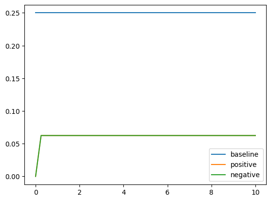
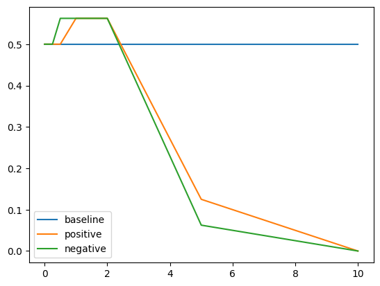
For rotten tomatoes, we see the expected performance gap of positive over negative, though positive does worse than no control. Moreover, we see in glue-wnli and sick, the negative control actually does better than positive control. In hate_speech18, we see the desired result.
Despite modifying the layers that we controlled, based upon observing the layers at which the Context Vectors had the most correlation to the trained concept, we cannot find a set of layers to control that works consistently across all four datasets, though we can find layers that work for one dataset.
Results for Control with Amplification
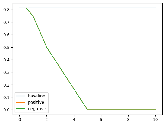
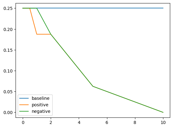
Note the result depends on the absolute value of $\alpha$ so the positive and negative graphs converge. The affect of amplification is quite smooth relative to addition in the sense that there is a consistent downward trend in performance for both amplification and suppression. This could be because amplification amplifies existing signals and this gets stronger as $\alpha$ increases.
Results for Control with Projection
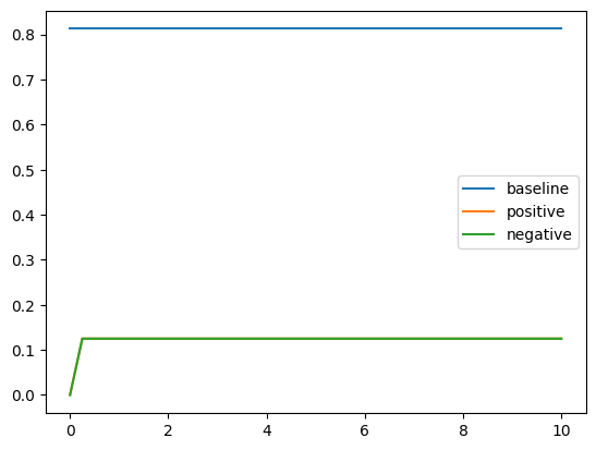
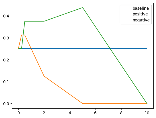
We can see that projection consistently decreases performance, which is expected as we can imagine projection as erasing the idea that the model needs to pay attention to these examples. Having positive or negative sign of $\alpha$ does not affect projection.
Ablation Studies
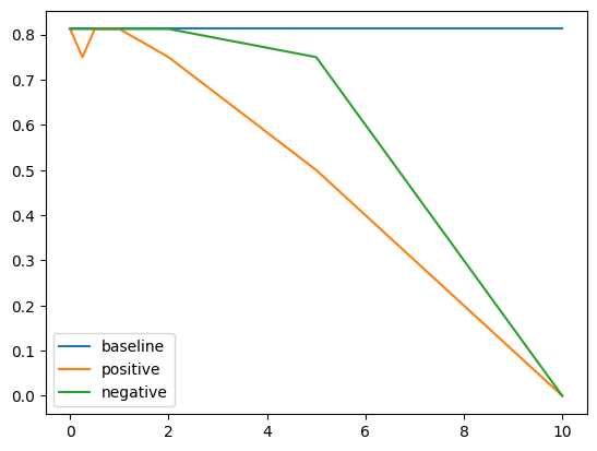
A key question is whether the Context Vectors are truly special. Especially because much of our results do not work, we would like to assess the “noise level.” By sampling a random unit vector from $4096$-dimensional space, the hidden dimension of Mistral-7b-instruct, for each layer and using that for control, we get the following results.
If we take the negative of all the Context Vectors, the graphs for positive and negative $\alpha$’s would switch. The fact that in our random sample we see such a large gap in the Glue-wnli graph indicates that there is quite a lot of noise. Moreover, if we take the negative of our particular randomly sampled vector, we obtain a Context Vector for Glue-wnli that is extremely good at controlling in-context-learning. The large landscape of $4096$-dimensional space is an exciting mystery.
Conclusion
While we understand our work is limited due to time and compute constraints and did not achieve the results we hoped for, we tried our best to explore this research direction of finding a Context Vector that corresponds to the in-context learning behaviors and experiments of using it to control model outputs.
Implications
If successful, this research direction could be a powerful tool to understand mechanistically why in-context learning emerges and potentially use model editing to achieve better State-of-the-Art results on LLMs in specific benchmark evaluation scenarios with model editing. Even with our current results that demonstrate more success in suppressing the Context Vector than amplifying it, i.e. suppressing such behaviors than boosting it, this can have implications on works that try to perform model unlearning and impact the robustness of LLMs.
Future Work
Through ablating with the random vector in the embedding space, it is unfortunate that controlling for the particular Context Vector we found is not particularly different from other vectors, despite it showing some promises on suppressing the results. We hope to run further ablation studies to confirm that suppressing the Context Vector is only suppressing the in-context learning behaviors of the specific behaviors and does not have other side effects.
Regarding our current setup of the contrasting prompts of telling the model to pay attention or not pay attention to the concept, we can further explore the space of contrasting prompts. Directly related to our work, we would also like to explore the other type of experiment setup in Zou et al. (2023)
We are also interested in exploring vectors that control step-by-step reasoning and in general, intelligence. The phrases “Let’s think step by step”