Can Constrastive Learning Recommend Me a Movie?
Introduction
With the vast amount of information and content available online, the need for intelligent recommendation systems has only become more necessary. Many of the apps we use, YouTube, TikTok, Instagram, Netflix, Spotify, etc. all incorporate recommender systems to provide personalized content. But how do these systems work? An important factor in delivering good recomendations is having a system that can find an expressive and useful representation of users and items (where items are the specific piece of content we want to recommend).
Traditional approaches for developing recommender systems include collaborative filtering, matrix factorization, and deep neural networks such as multi-layer perceptrons (MLPs) and graph neural networks (GNNs)
This project aims to explore if contrastive learning can be used to recommend movies for a user based on a their prior movie ratings.
More specifically, by choosing different strategies of defining positive/negative pairs, can we learn a user embedding that facilites the downstream task of movie recommendation?
Background And Related Work
Contrastive Learning
Contrastive learning is a self-supervised machine learning technique for training a model (often called an encoder) to distinguish between similar and dissimilar pairs of data points. The goal is to map each data point from its original representation space to a smaller dimensional latent space. If the encoder is trained well and is able to learn a good representation, the newly encoded data points should act as a sort of “compressed” version of the original data point while still containing some useful semantic information.
Contrastive learning has tradionally been used in the domains of computer vision and natural language processing. However, more recent work has shown that contrastive learning, when combined with graph neural networks (GNNs), can learn impressive representations when applied to recommender systems
Dataset
This project explores creating a movie recommender system based on the MovieLens dataset. The small version of this dataset contains 10,000 ratings of 9,000 movies by 600 users on a 0-5 star scale. Data was collected by users of the MovieLens website, last updated in September 2018. An example of the primary ratings.csv dataset is shown below:
| userId | movieId | rating | timestamp |
|---|---|---|---|
| 1 | 1 | 4.0 | 964982703 |
| 1 | 3 | 4.0 | 964981247 |
| … | … | … | … |
| 2 | 318 | 3.0 | 1445714835 |
| 2 | 333 | 4.0 | 1445715029 |
| … | … | … | … |
| 600 | 170875 | 3.0 | 1493846415 |
Methodology
Preprocessing of Dataset
The MovieLens dataset of user-movie interactions (movie ratings) is split into a training and test dataset. For each user, 95% of their interactions were randomly sampled and allocated to the training dataset, while the remaining 5% of interactions were allocated to the test dataset.
Thresholds were chosen to quantify whether a user “liked” a movie (LIKE_THRESHOLD) or “disliked” a movie (DISLIKE_THRESHOLD) based on that user’s rating. The training dataset was then filtered to only include interactions involving movies that had a minimum number of users who “liked” it and a minimum number of users who “disliked” the movie. This was to ensure that each movie had enough user data to facilite the computations for selecting positive / negative pairs.
Positive and Negative Pair Strategies
An important component of contrastive learning involves the definintion of positive pairs and negative pairs. For a given interaction (user u rates movie m), what should be considered a similar interaction and what should be considered a dissimilar interaction?
Given an interaction by user ${u}$, let $\text{pos}(u) = u^+$ and $\text{neg}(u) = u^-$ where $(u,u^+)$ is a positive pair and $(u,u^-)$ is a negative pair. The goal will be to find the pair of functions $\text{pos}(), \text{neg()}$ such that a good representation is learned.
Encoder Architecture
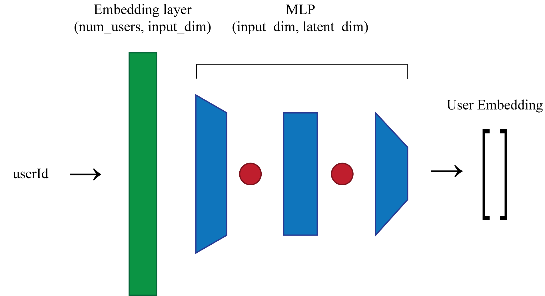
The proposed encoder architecture is shown below. The encoder recieves as input a batch of userIds, $u$ , integers in the range $0 \leq u \leq 599 $. The first layer of the encoder is an embedding layer, mapping userIds to a vector of dimension input_dim. This layer is followed by a 2-layer MLP with relu activations, with a hidden dimension of hidden_dim and an output dimension of latent_dim. Additionally, the final output of the encoder normalized.
Evaluation Metrics
In order to evaluate the quality of the learned user representations, there are a handful of metrics that will be used.
-
Top K Movie Recommendation: Movie recommendation will serve as a downstream task that acts as a proxy for how well the learned user representations are. To recommend movies for a user, the encoder is used to get the user embeddings for all users in the dataset. We then use the cosine-similarity to compute the N=10 nearest neighbors to our target user. From these N neighbors, we retreive all of their “liked” movies and sort by their respective ratings. The top K movies are returned as the system’s recommendations.
-
recall@k: A popular metric used for evaluating recommender systems is recall@k
. It measures the proportion of relevant items that were successfully retrieved from the top-k movie recommendations. Relevant items are defined as items that a user “likes” from the test dataset. The proportion of these items found in top-k recommendations from our recommender system (based on the learned encoder) is the recall@k. The higher the recall, the greater the overlap between our recommender’s recommended movies and the user’s actual preferred movies. -
Visualization of User Embeddings: By visualzing the learned user representation’s ability to be distinguished into separate clusters, we can better examine the potential user clusters for any distinguishing features. By utilizing t-distributed Stochastic Neighbor Embedding (TSNE) for dimensionality reduction of the user embedding vectors, we can project users representations to the 2D plane and use traditional clustering algorithms for visualization
. -
Top Movies Per User Cluster: To provide more insight into the resulting user embedding clusters, the top movies of the users in each cluster is also reported.
Experiments
In addition to standard hyperparamter-tuning techniques to optimize training, different positive pairs and negative pairs strategies will be tested.
All encoders were trained with num_epochs = 20, batch_size = 512, lr = 0.0001 (using Adam optimizer), and contrastive triplet loss.
Strategy 1
For a given user $u_i$ a similar user is determined by a random selection from a set of candidate users. These candidate users consist of the subset of users that have “liked” the same movies that $u_i$ “liked”, i.e. their ratings $\geq$ LIKE_THRESHOLD. Likewise, dissimilar users for $u_i$ were randomly selected from a set of candidate users that “disliked” the same movies $u_i$ “disliked”, i.e. their ratings $ < $ DISLIKE_THRESHOLD.
| LIKE_THRESHOLD | DISLIKE_THRESHOLD |
|---|---|
| 3.5 | 3.5 |
With these definitions of positive and negative pairs, an encoder was trained with the resulting user embeddings shown below.
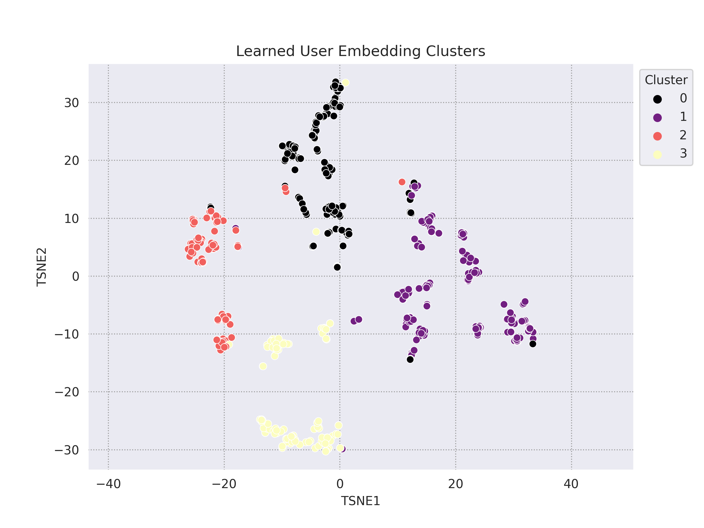
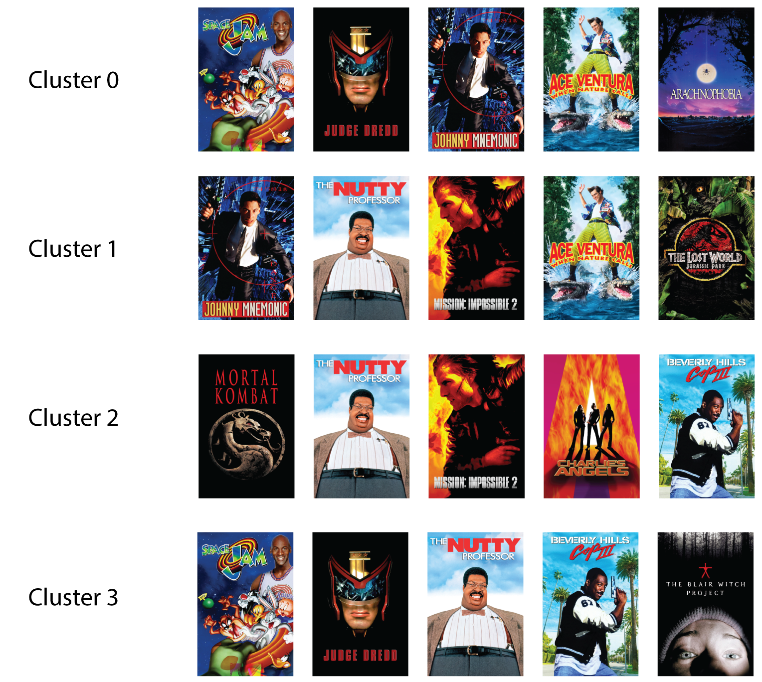
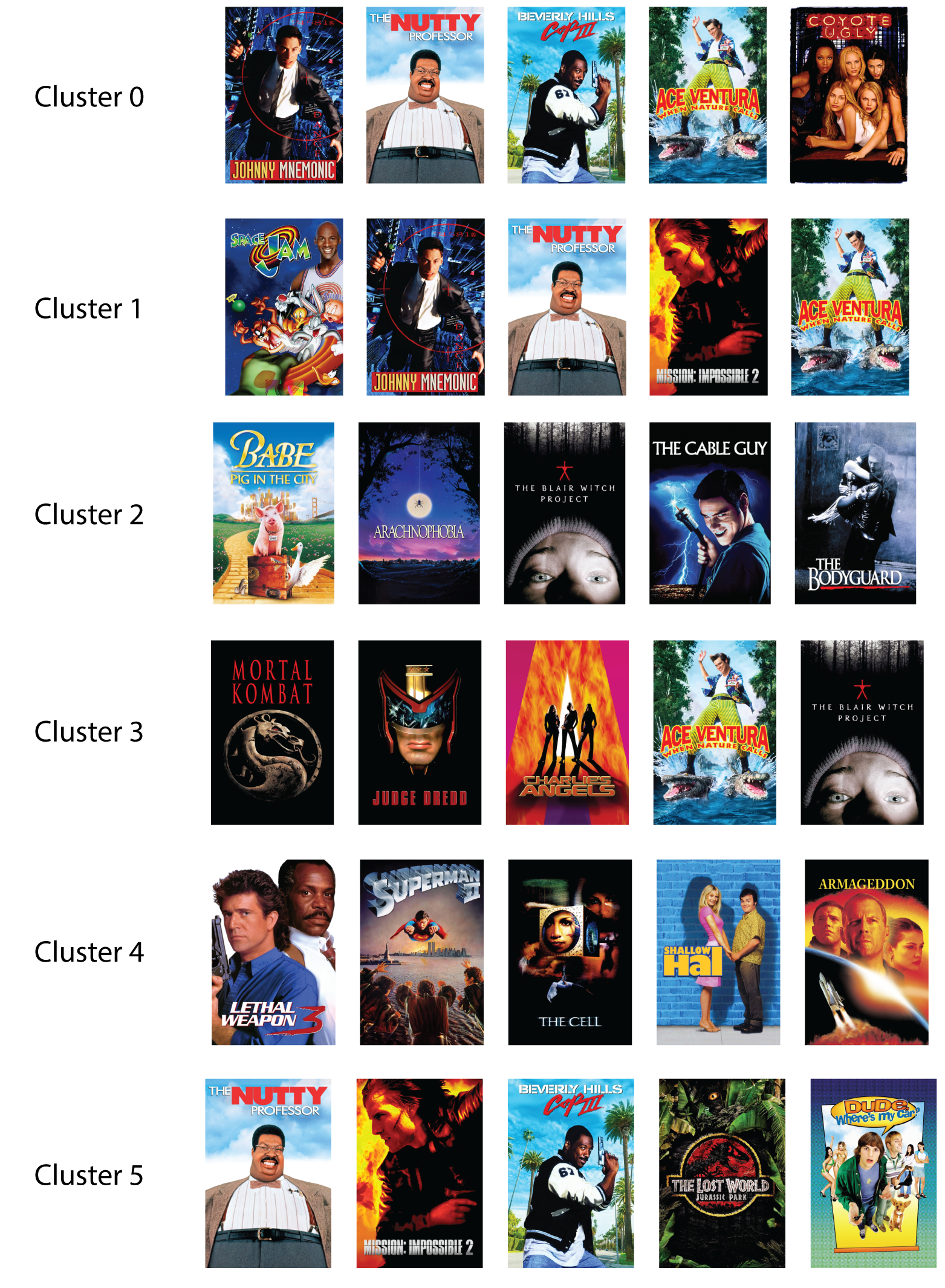
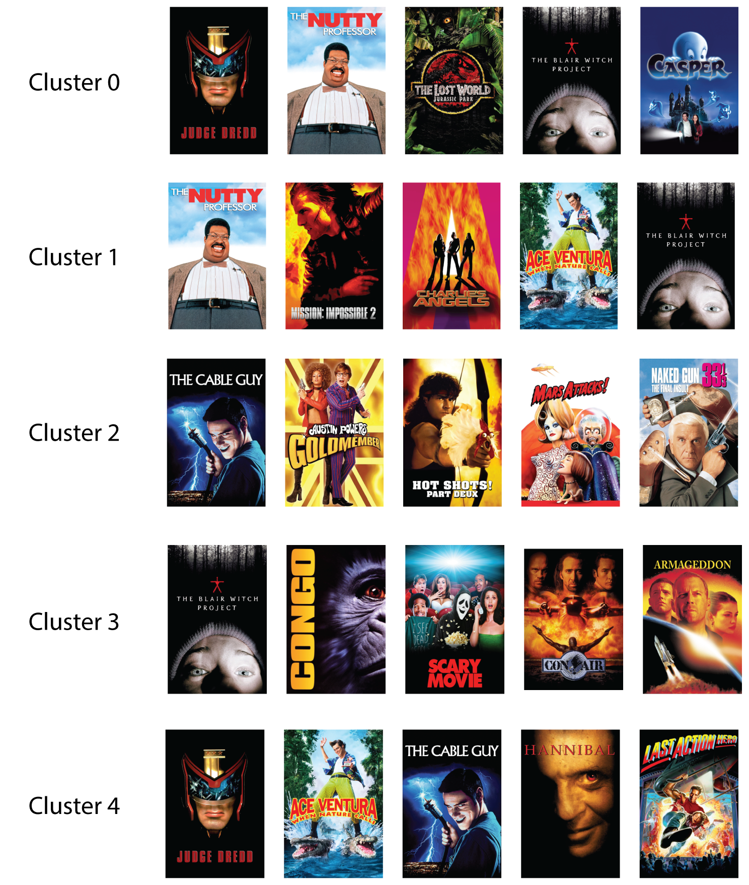
By examining the user embedding clusters, we see four loosely-defined user clusters. The top 5 highest rated movies by each cluster’s members are also depicted. A key takeaway is that we see a repetition of the same movies across each cluster, movies like The Nutty Professor, Mission Impossible 2, Ace Ventura: When Nature Calls, etc. These are all very popular and well-liked movies with a wide audience. The prevalence of highly-rated and popular movies such as these leads to a bias in our positive pairs. Since many users are fans of these movies, they are all considered similar users, i.e. our definition of similarity is too weak. The following strategies will try to address this.
Strategy 2
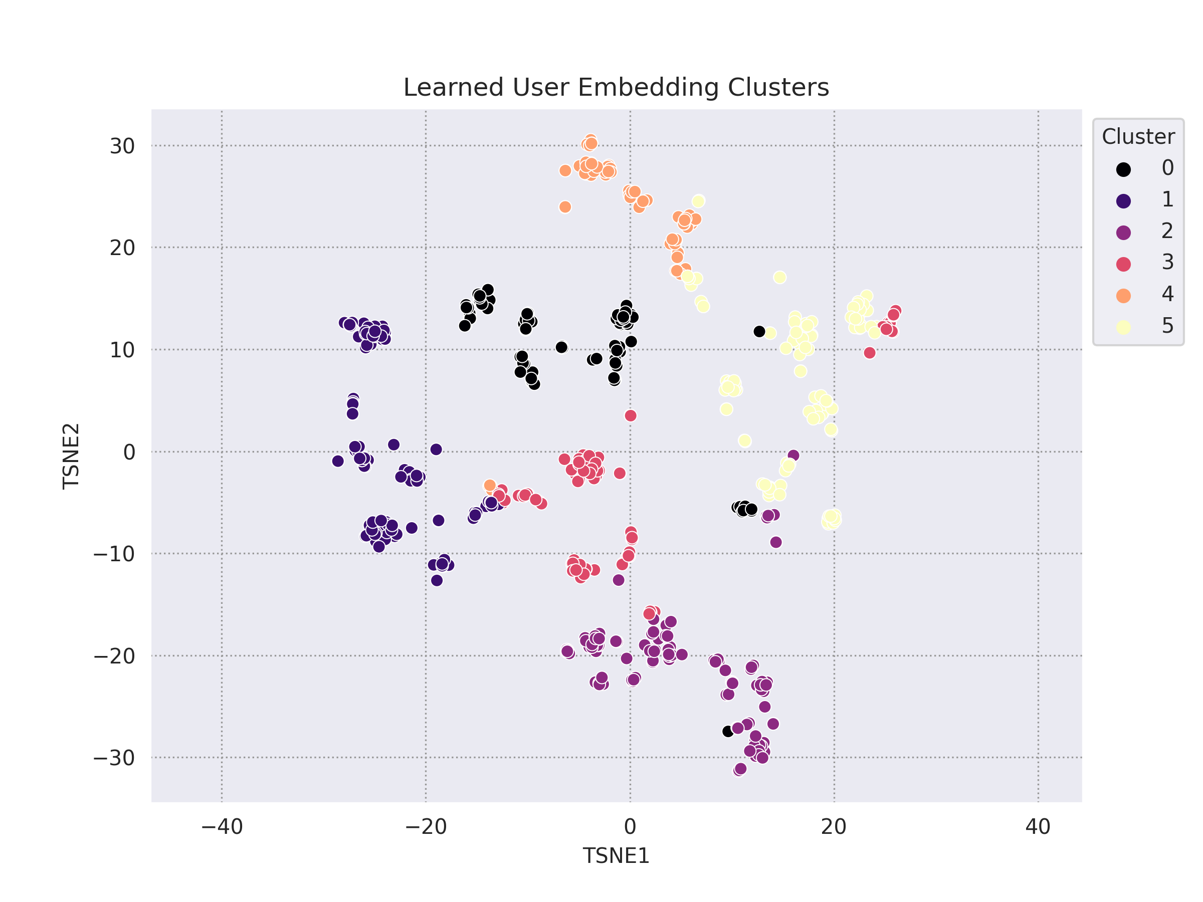
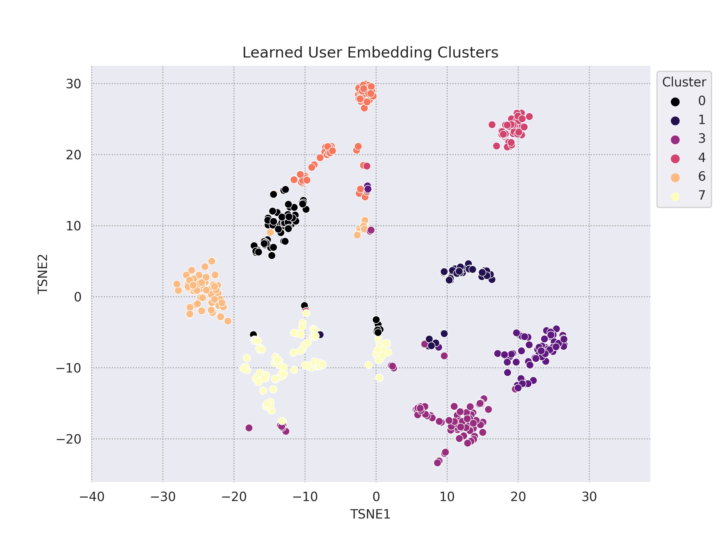
In order to decrease the influence of popular movies, one strategy is to filter out all movies that are “liked” by a certain number of users. We define POPULARITY_THRESHOLD = 100, which removes all movies with over 100 “liked” users. As a result, the distribution of “liked” users per movie is relatively uniform. The definitions of positive and negative pairs remains the same as in Strategy 1.
| LIKE_THRESHOLD | DISLIKE_THRESHOLD |
|---|---|
| 3.5 | 3.5 |
Strategy 3
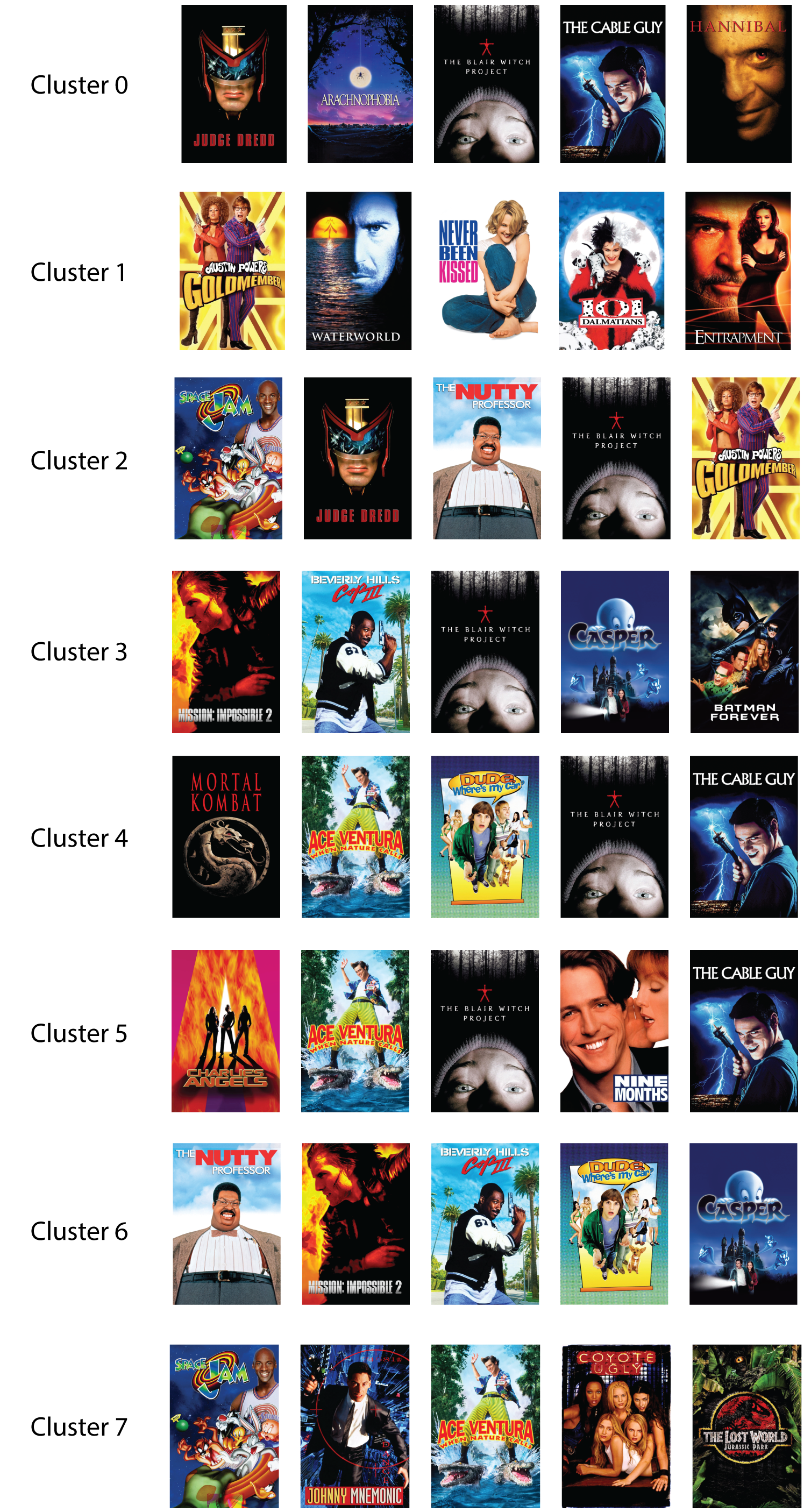
A different method for reducing the influence of popular movies was to normalize each users ratings. By subtracting a movie’s average rating across all users from any particular user’s rating, we are able to determine whether the user liked the movie more than others or disliked it more than others. Popular movies only have an impact if the user really liked (or disliked) it relative to everyone else.
Using this new strategy, for any user $u_i$, instead of randomly selecting a similar user from candidates that “liked” a movie in common, these candidate users are ranked such that the candidate that has the highest normalizes rating is selected (the opposite is true for choosing a disimilar user). Therefore, instead of having a positive pair of users who rated the same movie highly, the positive pair will consist of users who both gave the same movie a higher rating than the average user.
| LIKE_THRESHOLD | DISLIKE_THRESHOLD |
|---|---|
| 3.5 | 3.5 |
Strategy 4
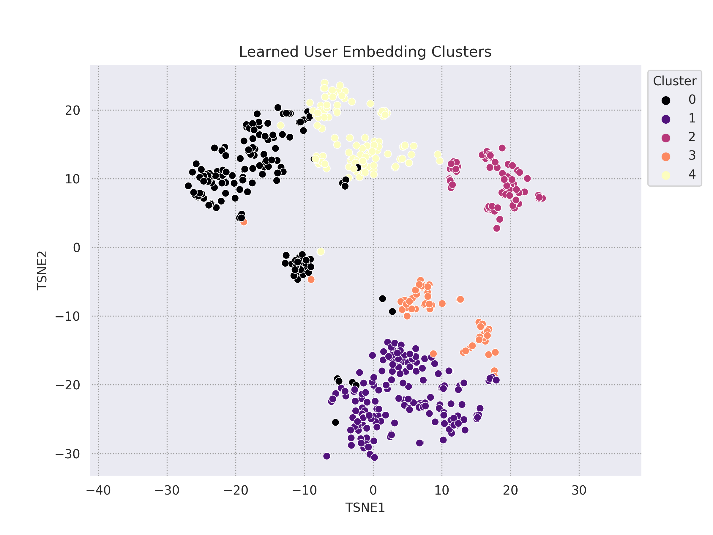
Despite the previous strategies, there still seems to be a lack of cohesion among the resulting user embedding clusters. The final strategy tested was a hybrid approach. In this scenario, the LIKE_THRESHOLD has been raised and the DISLIKE_THRESHOLD lowered in an attempt to narrow the candidate pools to more extreme users. Moreover, Strategies 2 and 3 are combined. Highly popular movies are removed and normalized ratings are used.
| LIKE_THRESHOLD | DISLIKE_THRESHOLD |
|---|---|
| 4 | 3 |
Analysis
For each strategy, the recall@k for various values of k are shown, along with the sizes of the train and test datasets after filtering.
| Strategy 1 | Strategy 2 | Strategy 3 | Strategy 4 | |
|---|---|---|---|---|
| recall@10 (%) | 0.62 | 1.29 | 0.73 | 0.78 |
| recall@20 (%) | 1.97 | 2.16 | 2.18 | 3.10 |
| recall@50 (%) | 3.84 | 6.03 | 4.36 | 11.63 |
| Size Train Set | 51,576 | 32,609 | 51,576 | 10,826 |
| Size Test Set | 1,361 | 984 | 1,361 | 232 |
It appears that both Strategy 2 and Strategy 3 alone seemed to make a noticable improvement in recall, with Strategy 2 (the removal of the most popular movies) making a larger impact than normalizing ratings. Furthermore, by using both strategies along with a few other changes, a representation the resulted in a better recomender system and more well-defined embedding clusters was learned.
Conclusion
From the above experiments, it seems that contrastive learning (even when used with a simple MLP encoder) can eventually learn a user embedding resulting in clusters. However, it seems like either a more advanced architecture or positive/negative pair mining procedures are required to ensure that the learned representations have a useful semantic meaning. Weak positive pairs resulted from the presence of popular movies with diverse audiences. Previous work in applying contrastive learning to recommender systems highlight more complex formulations of ranked loss functions, assigning different weights depending on whether the pairs are hard or easy negative samples
An interesting extension of this project could explore the use of GNNs as the basis of the encoder architecture, as these types of models more naturally preserve the structure of user-movie interactions.