Quantum Circuit Optimization with Graph Neural Nets
We perform a systematic study of architectural choices of graph neural net-based reinforcement learning agents for quantum circuit optimization.
Introduction
One of the most notable technological developments of the past century has been computing based on binary bits (0’s and 1’s). Over the past decades, however, a new approach based on the principles of quantum mechanics threatens to usurp the reigning champion. Basing the informational unit on the quantum bit, or qubit, instead of the binary bit of “classical” computing, quantum computing takes advantage of the strange phenomena of modern physics like superposition, entanglement, and quantum tunneling.
Leveraging these as algorithmic tools, surprising new algorithms may be created. Shor’s algorithm, based on quantum algorithms, can solve classically hard cryptographic puzzles, threatening the security of current cryptographic protocols. Additionally, quantum computers can significantly accelerate drug discovery and materials science through quantum molecular dynamics simulations. They also show great potential in Quantum Machine Learning (QML), enhancing data analysis and pattern recognition tasks that are computationally intensive for classical computers.
Similar to classical computers, which base their algorithms on circuits, quantum computers build their quantum algorithms on quantum circuits. However, quantum computers are still in development and are incredibly noisy. The complexity of a quantum circuit increases its susceptibility to errors. Therefore, optimizing quantum circuits to their smallest equivalent form is a crucial approach to minimize unnecessary complexity. This optimization is framed as a reinforcement learning problem, where agent actions are circuit transformations, allowing the training of RL agents to perform Quantum Circuit Optimization (QCO). Previous techniques in this domain have employed agents based on convolutional neural networks (CNN)
My previous research has demonstrated that the inherent graphical structure of circuits make QCO based on graph neural networks (GNN) more promising than CNNs. GNNs are particularly effective for data with a graph-like structure, such as social networks, subways, and molecules. Their unique property is that the model’s structure mirrors the data’s structure, which they operate over. This adaptability sets GNNs apart from other machine learning models, like CNNs or transformers, which can actually be reduced to GNNs. This alignment makes GNNs a highly promising approach for optimizing quantum circuits, potentially leading to more efficient and error-resistant quantum computing algorithms.
This project extends my previous work by systematically investigating the impact of various architectural choices on the performance of GNNs in quantum circuit optimization. This is achieved through a series of experiments focusing on key variables such as the number of layers in the GNN, the implementation of positional encoding, and the types of GNN layers used.
Specific objectives include:
- Evaluating the Number of GNN Layers: Investigating how the depth of GNNs influences the accuracy and efficiency of quantum circuit optimization. This involves comparing shallow networks against deeper configurations to understand the trade-offs between complexity and performance.
- Exploring Positional Encoding Techniques: Positional encoding plays a crucial role in GNNs by providing information about the structure and position of nodes within a graph. This project experiments with various encoding methods to determine their impact on the accuracy of quantum circuit optimization.
- Assessing Different Sizes of Hidden Dimension: This objective focuses on understanding the influence of the hidden dimension size within GNN layers on the performance of quantum circuit optimization. By varying the size of the hidden dimension, the project identifies the optimal balance between computational complexity and the model’s ability to capture complex relationships within the data.
Quantum Circuits and Transformation Environment
In order to have quantum circuit optimizers we need quantum circuits! Quantum circuits are built out of quantum gates operating on qubits. These quatum circuits implement quantum algorithms in a similar way that classical circuits implement classical algorithms. In the below example, we have a five qubit circuit. It has a variety of single qubit gates (X, Rz, and H) as well as two qubit gates (CX).

Some gates have classical analogs, like the X gate which is analogous to the classical NOT bit-flip gate. Others, like the Hadamaard (H) gate, cannot be understood with classical intuition. We can use gates like H in combination with a two qubit gate like CX two put two qubits into unique quantum states. For example, with the following circuit, we can put two qubits into a special state called “quantum entanglement”.
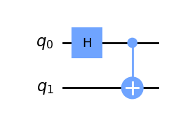
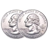
These qubits have outcomes that are perfectly correlated with each other. If they are measured, they will always result in the same outcome, even if after the circuit is applied the qubits are separated an arbitrary distance. This is despite the fact that the outcome is perfectly random! Measurement will result in 0 and 1 with probability 50% each. This is like flipping two coins whose outcome you cannot predict, but which always land both heads or both tails.
We can write the circuit and subsequent quantum state with the following equation. The two possible resulting states (both heads or both tails) are represented in bracket notation: \(\ket{00}\) and \(\ket{11}\).
\begin{equation} \ket{\psi} = \text{CX} \cdot (H \otimes I) \ket{00} = \frac{1}{\sqrt{2}}(\ket{00} + \ket{11}) \end{equation}
However, just like classical algorithms can be written down according to different programs and circuits which do the same thing, quantum circuits can have different equivalent forms. Transitions between these equivalent forms can be written down according to a set of local rules mapping from some set of quantum gates to another.
In the following diagram we show the quantum transformations used for this project. They are ordered according to 1) single qubit, 2) two qubit, and 3) three qubit transformations.
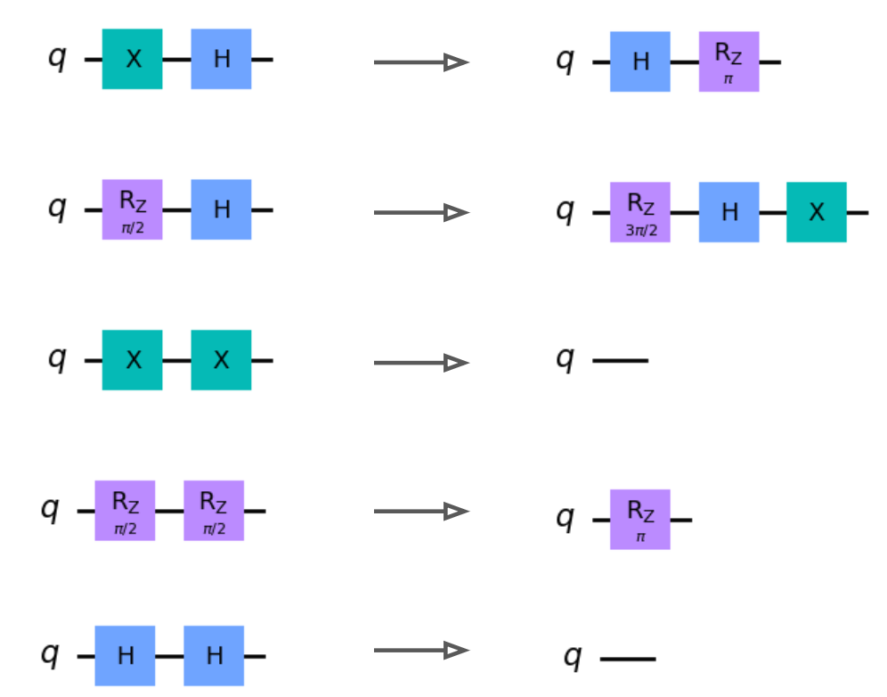
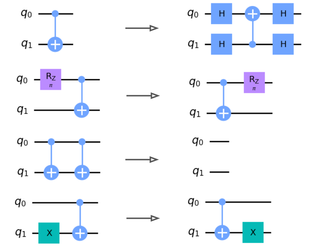
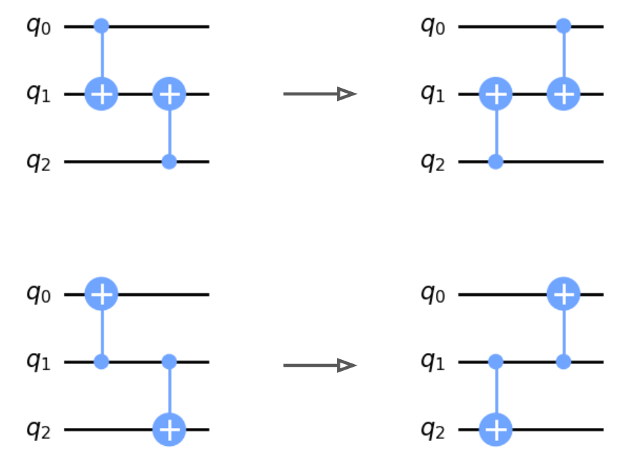
These transformations will serve as the action space for our quantum circuit environment. Notably, some of these circuit transformations involve merges or cancellations, which can be used to simplify the circuits. A quantum agent which chooses an appropriate sequence of circuit transformations can then simplify a circuit into an equivalent form with fewer gates. Therefore, the task of circuit optimization may be decomposed into a trajectory of agent steps leading between different states, where states correspond to quantum circuits which are all algorithmically equivalent.
Proximal Policy Optimization
To train the GNN agent, we use the Proximal Policy Optimization (PPO) algorithm. PPO is a model-free, on-policy reinforcement learning algorithm that aims to optimize the policy of a reinforcement learning agent by iteratively updating its policy network. We train the GNN agent on n-qubit random circuits. For training the GNN-based agents for quantum circuit optimization, we use the Proximal Policy Optimization (PPO) algorithm. PPO is a deep reinforcement learning algorithm that has shown success in a variety of applications, including game playing and robotics. The algorithm updates the policy by maximizing a surrogate objective function that approximates the expected improvement in the policy, while enforcing a constraint on the maximum change in the policy. This constraint helps to prevent the policy from changing too much from one iteration to the next, which can destabilize the training process.
\begin{equation} L^{\text{CLIP}}(\theta) = \hat{\mathbb{E}}_t[\min(r_t(\theta))\hat{A}_t, \text{clip}(r_t(\theta), 1 - \epsilon, 1 + \epsilon)\hat{A}_t] \end{equation}
To train the GNN agents for quantum circuit optimization, we start by initializing the GNN weights randomly. We then use the PPO algorithm to update the weights by sampling circuits from a distribution of n-qubit random circuits, encoding them into graphs, and simulating the circuits in a custom python gym environment. For each transformation we use
\begin{equation} r_t = - \left(q(s_{t+1}) - q(s_{t})\right) \end{equation}
as the reward signal for the PPO algorithm following
We use \(q(s) = -\texttt{circuit_size}(s)\), such that the agent’s objective is to reduce the overall circuit size, as measured by number of gates, resulting in the reward function:
\begin{equation} r_t = \texttt{circuit_size}(s_{t+1}) - \texttt{circuit_size}(s_t) \end{equation}
The methodology for implementing the quantum circuit optimization using deep reinforcement learning and graph neural networks consists of three main components: (1) encoding the circuits as directed acyclic graphs using the DAG encoding and (2) encoding the graphs as node and edge feature tensors and training a GNN-based agent using the PPO algorithm,.
GNN architecture
The GNN architecture used is inspired by the message passing neural network (MPNN), which is a type of GNN that performs iterative message passing between nodes in the graph. The GNN architecture used for this approach consists of \(L\) layers of Residual Gated Graph ConvNets.

The GNN gets as input the graph (encoded as the three tensors shown above), the positional encoding, and a binary tensor encoding of which transformations are allowed for each node (this can be computed in \(O(\# nodes)\) time).
Node features and positional encoding are both mapped to a k-dimensional embedding with a linear transformation and concatenated added together, forming a vector \(h\). The edge features are also linearly mapped to some \(l\)-dimensional embedding vector \(e\).
After, passing through \(L\) layers, each node has a feature vector \(h’\). These features are mapped to a length \(t\) Q-vector where t=# transformations. A mask is applied so that all impossible transformations are ignored. The length \(t\) Q-vectors are concatenated together from all nodes and then outputted by the GNN. An action is selected by choosing the node/transformation which corresponds to the index of the maximum Q-value.
Results
After training our graph neural network agent in the quantum circuit environment using PPO, we can verify that the agent can indeed optimize circuits. We randomly sample a five qubit circuit and run our agent on the circuit for fifty steps. We see that the agent is able to successfully reduce the cirucit size from 44 gates to 30, a 14 gate reduction. Meanwhile, the standard Qiskit optimizer could only reduce the circuit to 36 gates.
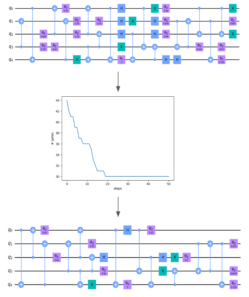
Now that we have verified our learning algorithm we can successfully train a quantum circuit optimizing agent, we proceed with our study over three hyperparameters: 1) number of layers, 2) the use of positional encoding, and 3) hidden dimension. For all plots, we display the average over several runs with standard error.
Number of Layers
We innvestigate how the depth of GNNs influences the accuracy and efficiency of quantum circuit optimization. This involves comparing shallow networks against deeper configurations to understand the trade-offs between complexity and performance. In order to do this we scan over the number of layers \(L\) in our GNN from 1 to 7.
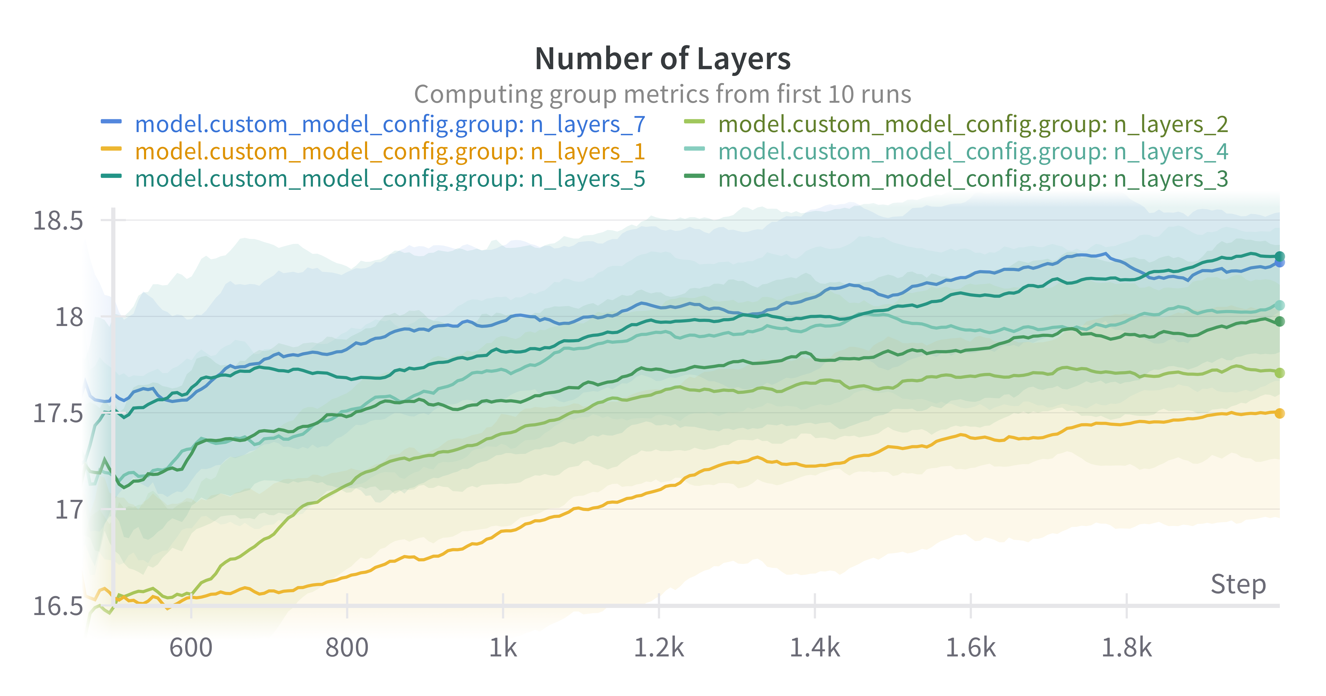
We see that, generally, increasing the number of layers in the model improves performance of the model on random circuits. This is aligned with the intuition that increasing the number of layers of a GNN allows models to “see” information from further away, which can be used to make strategic decisions.
However, we also observe that there is some critical point in which increasing \(L\) no longer leads to better outcomes from the model. This threshold appears to occur around \(L=5\), which performs similarly to \(L=7\).
This could be related to a known property of GNNs, in which features of nodes which are closer together are more similar. This becomes excerterbated as the number of layers increase, smearing out information. Therefore, we expect that if we continued to increase \(L\) then model performance would degrade.
Positional Encoding
Positional encoding can provide information about the structure and position of nodes within a graph. These features can often play a role in symmetry-breaking.
In addition to the existing features encoding gate type and wire information, we concatenate 8 normally distributed dimensions to the feature vector. We hypothesize that these random features can be used to “ID” gates that have the same gate type but are a located in different locations. We experiment with training a GNN with and without the addition of random positional encoding.
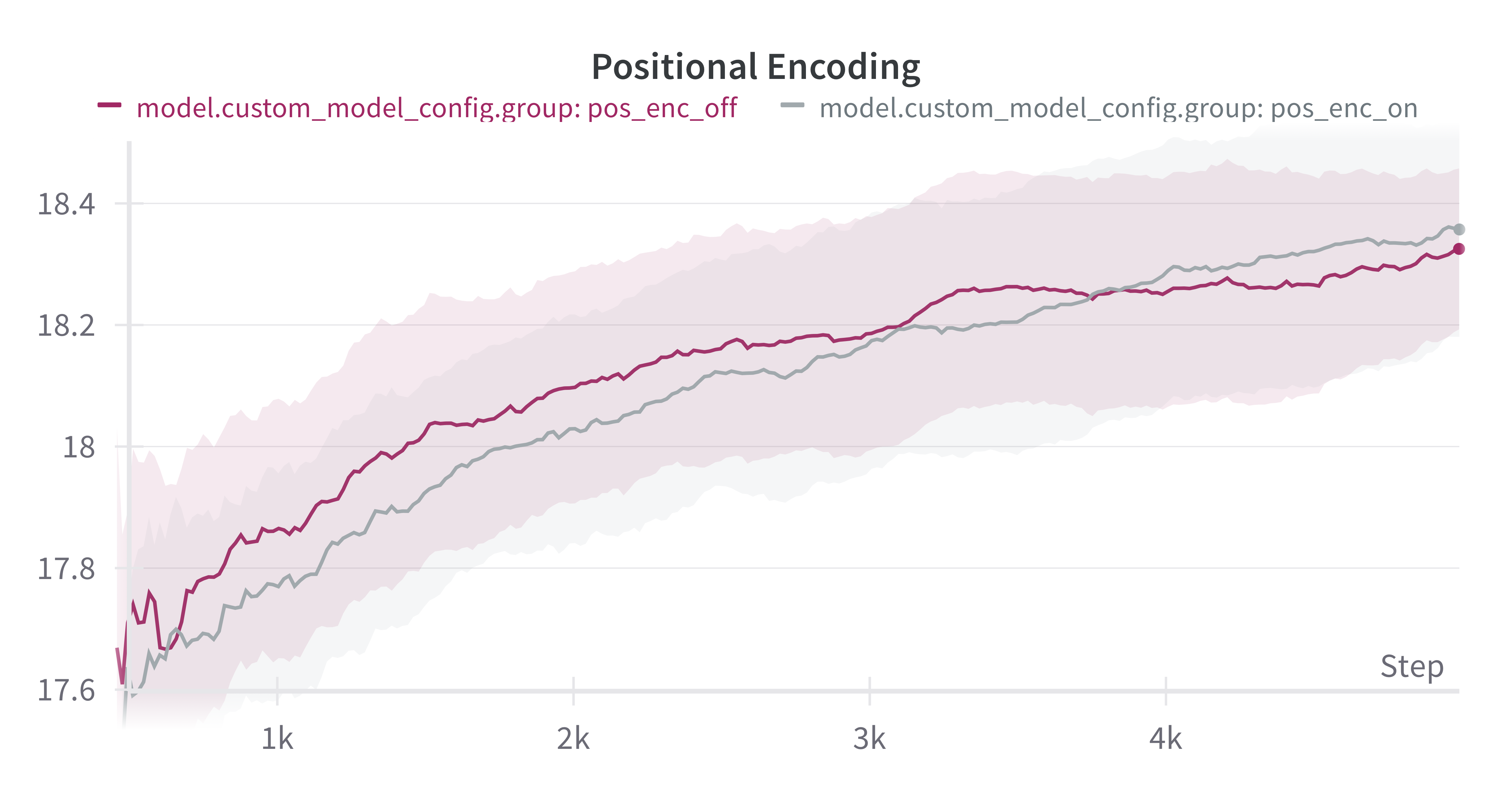
The resulting plot shows inconclusive evidence. While the random positional encoding came out on top at the end of training, the difference is not significant enough to be able to conclude that it is demonstrably better.
Hidden Dimension
The last hyperparameter we examine is the hidden dimension of the GNN layers. We scan over values 16, 32, 64, and 128. All other parameters are kept fixed.
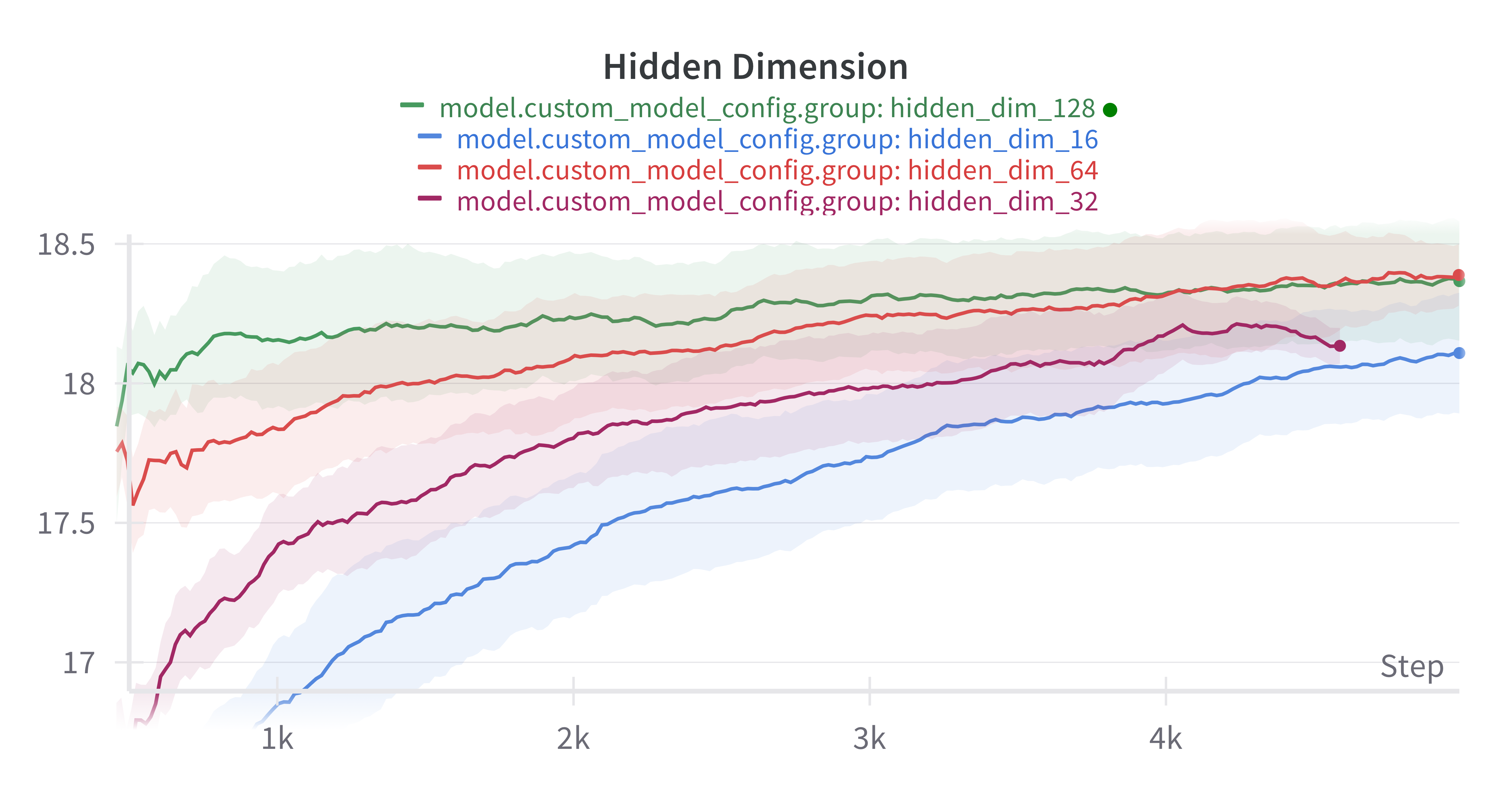
We observe that performance tends to improve with scale. However, similarly to the “number of layers” hyperparameter, there appears to be some critical threshold after which scaling no longer appears to improve performance. From our experiments this threshold appears to be around 64.
It is unclear what would happen if we continued scaling past 128. For example, the performance could stay at the plateau reached at hidden dimension 64 and 128, or it could eventually get worse.
Further Work
While this work gave a first glimpse at some of the structural properties that work with GNNs for RL on quantum circuits, much remaining work remains.
Notacably, many of the training runs did not seem to train until plateau. To be fully confident in the results, training until plateau would be necessary for full confidence. Additionally, many of the runs were quite noisy, making it difficult to distinguish between the performance under different runs. Therefore, increasing training samples could effectively reduce standard error for better statistics.
Moreover, the scope of future exploration can be expanded. One of the most interesting areas of future work would be on what types of graph layers work best. While we use Residual Gated Convulation Nets, it is not clear that this is the best layer type. Other things than could be tested are other positional encoding schemes. While we experimented with random features, more standard positional encoding schemes include Laplacian and Random walk encoding.
Conclusion
We find that there appears to be critical thresholds of optimal values for the hidden dimension and number of layers in GNNs. We also find no evidence that random positional encoding appears to improve performance, contrary to intuition that it would serve a useful symmetry-breaking function. While much work is left to be done, this work provides a first investigation into how performance of GNNs on QCO can be affected by various choices of hyperparameters.