Using Synthetic Data to Minimize Real Data Requirements

Data acquisition for some tasks in synthetic biology can be cripplingly difficult to perform at a scale necessary for machine learning... so what if we just made our data up?*

*And used it as the basis for transfer learning with the real data that someone put hard work in to generate.

Introduction

Synthetic biology is a burgeoning field of research which has attracted a lot of attention of the scientific community in recent years with the advancement of technologies that enable the better understanding and manipulation of biological systems. A significant contributor to its steadily increasing popularity is the diverse array of potential applications synthetic biology may have, ranging from curing cancer, to addressing significant climate issues, to colonizing other planets. But, to effectively manipulate these biological systems, it is necessary to understand how they work and how they interact with other biological systems — it has been shown time and time again that a system characterized in isolation, compared to the same system in a broader, non-isolated context, will not perform identically. This necessitates models that can predict a system’s behavior given both stimuli and context.

In the synthetic biology literature, the behavior of many systems is characterized by the chemical reactions that take place; these reactions consist most frequently of the so-called central dogma of biology, in which DNA produces RNA, which produces proteins. These proteins are then free to perform almost every function within a cell, including — most notably for us — regulation of DNA. By varying the extent and nature of this regulation, these systems yield mathematical models that range from simple linear systems to highly complex nonlinear dynamical systems:

Figure 1: A simple model of the central dogma of biology: a stretch of DNA is used to create a strand of messenger RNA, which is used to create a functional protein. Functional proteins are responsible for almost all operations within the cell, from cellular movement to RNA production and everything in between.

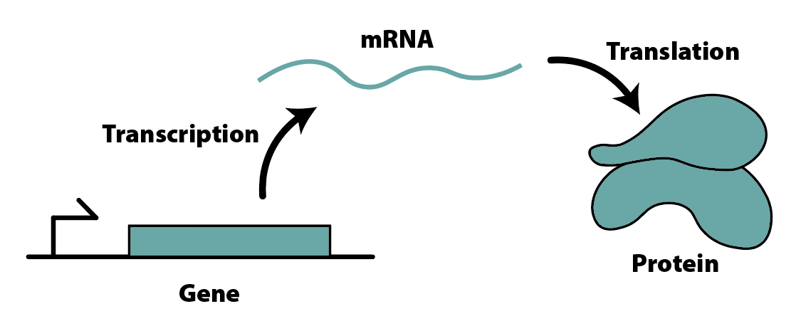
However, the figure above does not capture the full purview of the cell; it neglects factors that synthetic biologists know to be critical to the process of protein expression, as well as factors that have not been characterized rigorously yet. The process of analyzing the behavior of a system at the fullest level of detail necessary to encapsulate these intricate dynamics is expensive and time-consuming, and requires significant experimental data to validate — not to mention the fact that, as was mentioned, there are some factors which we simply don’t know about yet. Protein production is an immense and complex task, and identifying its critical parameters at the highest level of detail is no small feat.

Enter Machine Learning

With this in mind, many synthetic biologists are experimenting with characterizing system behavior, especially when augmenting pre-existing models to include newly discovered phenomena, using machine learning and neural networks, due to their universal function approximator property. In this fashion, we may be able to better abstract the levels of biological detail, enabling better prediction of the composition of two genetic circuits.

Unfortunately, training neural networks also requires (surprise surprise!) substantial experimental data, which is taxing on both a researcher’s budget and time — for a small lab with few researchers working, a single experiment may take upwards of 12 hours of attentive action, while yielding only up to 96 data points for training. Some large-scale gene expression data has been collected to assist in the development of machine learning algorithms; however, this data is focused largely on the expression of a static set of genes in different cellular contexts — rather than on a dynamic set of genes being assembled — and is therefore insufficient to address the questions of composition that are being posed here.

This leads us to a fundamental question: can we use transfer learning to reduce the experimental data we need for training by pre-training on a synthetic dataset which uses a less-detailed model of our system? In other words, can we still derive value from the models that we know don’t account for the full depth of the system? If so, what kinds of structural similarities need to be in place for this to be the case?

In this project, we aim to address each of these questions; to do this, we will first pre-train a model using simpler synthetic data, and use this pre-trained model’s parameters as the basis for training a host of models on varying volumes of our more complex real data. Then, we will consider sets of more complex real data that are less structurally similar to our original synthetic data, and see how well our transfer learning works with each of these sets.

In theory, since the synthetic data from the literature uses models that have already captured some of the critical details in the model, this fine-tuning step will allow us to only learn the new things that are specific to this more complex model, thus allowing transfer learning to be successful. As the two underlying models become increasingly distant, then, one would expect that this transfer will become less and less effective.

Methods

Problem Formulation

Consider we have access to a limited number of datapoints which are input-output $(x_i,y_i)$ pairs for a biological system, and we want to train a neural network to capture the system behavior. The experimental data for the output $y_i$ we have is corrupted by an additive unit gaussian noise, due to white noise and measurement equipment precision. Moreover, we consider that we also have access to a theoretical model from another biological system which we know to be a simplified version of the one in our experiments, but which explicitly defines a mapping $\hat y_i = g(x_i)$.

Our goal is thus to train a model $y_i = f(x_i)$ to predict the real pairs while using minimal real pairs of data $(x_i, y_i)$. Instead, we will pre-train with $(x_i, \hat y_i)$ pairs of synthetic data, and use our real data for fine-tuning.

Data Acquisition

In this work we will additionally consider a domain shift between two datasets, which we will refer to as the big domain and the small domain. In the big domain, our inputs will vary between 0 and 20nM, and in the small domain the inputs will vary between 0 and 10nM. These domains represent the ranges for the inputs in the experiments in the small domain, which may be limited due to laboratory equipment, and the desired operation range of the systems in the big domain.

Furthermore, for all datasets - pre-training, fine-tuning, or oracle training - we will be generating synthetic data for training and testing purposes. We will use different levels of complexity to simulate a difference between experimentally-generated and computationally-generated data. In a real setting, we would use the complex model $f$ that we’re trying to learn here as the simple, known model $g$ in our setup. Going forward, we will refer to the data generated by our low-complexity model $g$ as “synthetic” data, and to the data generated by our high-complexity model as “real” or “experimental” data.

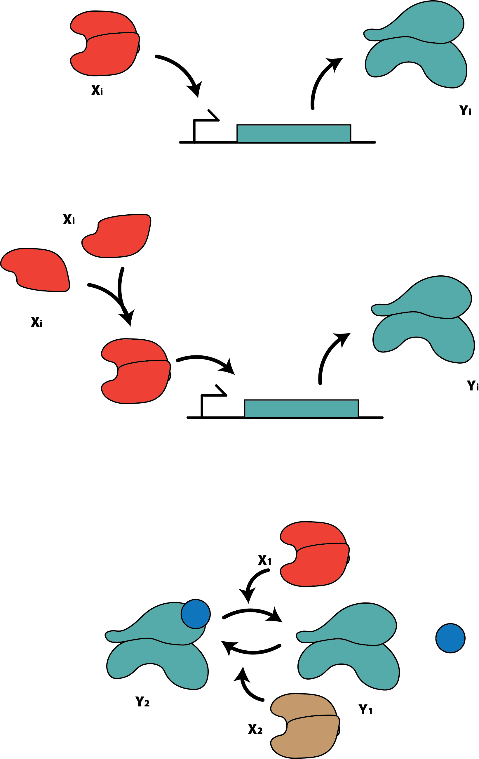
For our low-complexity theoretical model, we consider the simplest gene expression model available in the literature, in which the input $x_i$ is an activator, and the output $y_i$ is given by the following Hill function:

\[y_i = \eta_i \frac{\theta_i x_i}{1 + \Sigma_{j=1}^2 \theta_j x_j}, i\in {1,2},\]

where our $\eta_i$’s and $\theta_i$’s are all inherent parameters of the system.

For the first experimental model, we consider a more complex gene expression model, where the activator $x_i$ must form an $n$-part complex with itself before being able to start the gene expression process, which yields the following expression for the output $y_i$:

\[y_i = \eta_i \frac{(\theta_i x_i)^n}{1 + \Sigma_{j=1}^2 (\theta_j x_j)^n}, i\in {1,2},\]

where - once again - our $\eta_i$’s and $\theta_i$’s are all inherent parameters of the system. Note that, at $n=1$, our real model is identical to our synthetic model. As one metric of increasing complexity, we will vary $n$ to change the steepness of the drop of this Hill function.

As an additional test of increased complexity, we will consider a phosphorylation cycle in which inputs $x_i$ induce the phosphorylation or dephosphorylation of a given protein. We take the dephosphorylated protein to be an output $y_1$, and the phosphorylated protein to be a secondary output $y_2$, for which we have:

\[y_i = y_{tot} \frac{\theta_i x_i}{\Sigma_{j=1}^2 \theta_j x_j}, i\in {1,2},\]

in which $\theta_i$’s and $y_{tot}$ are each system parameters. Note that the only functional difference between this system and the synthetic data generation system lies in the denominator of each, as one has a nonzero bias term, where the other does not.

Figure 2: Graphical representation of the three different synthetic or experimental models used in this project. In the first diagram, our input protein $x_i$ is activating the production of an output protein $y_i$. This is the simplest model of which we can conceive, and constitutes our synthetic data. In the second diagram, two copies of our input protein $x_i$ come together to form a complex that induces the production of our output protein $y_i$. This is a step up in complexity, and varying the number of proteins that come together allows us to introduce more and more complexity into our system. Finally, a single protein which can be either of our outputs $y_1$ or $y_2$ is moved between these states by our two input proteins $x_1$ and $x_2$. This system, while seemingly very dissimilar from the above two, winds up being mathematically not too far off, and offers another model on which to transfer our learning.

Training & Testing

For each experiment, we trained MLPs composed of 5 hidden layers with 10 nodes each and a ReLU activation function.

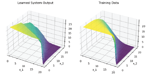
For the first experiment, we performed transfer learning by pre-training our model for 90% of the total number of epochs (1800/2000) with the synthetic data sampled from the big domain, where we have a high quantity of data points (40000 $(x_i, y_i)$ pairs); for the remaining 10% of epochs, the network was trained on the experimental data sampled from the small domain, with varying numbers of data points used for training. This can be compared to a model trained exclusively on the same volume of experimental data for a full 2000 epochs, to establish a baseline level of performance. An oracle model was trained for all 2000 epochs on experimental data sampled from the big domain with a high volume of data, and serves as the best-case performance of our model.

For the second experiment, we followed a very similar protocol as in the first experiment; the critical difference here lies in the fact that, where the fine-tuning step used different volumes of data in the previous case, we now instead use a fixed data volume (1000 $(x_i, y_i)$ pairs), and fine-tune on a host of different models of varying complexity relative to the synthetic model.

To evaluate performance of our neural networks, we uniformly sample 100 points from the big domain, for which we calculate the L1 loss mean and variance between the network predictions and the experimental model output.

Figure 3: A visual example of the training done - on the right is the intended function to be learned, where the left features the output of one of the models that was trained with transfer learning.

Results & Analysis

Experiment 1

As was mentioned before, the first experiment was targeted towards addressing the question of whether we can pre-train a model and use transfer learning to reduce the volume of real data needed to achieve a comparable standard of accuracy. To this end, we trained several models with a fixed volume of pre-training data, and varied the volume of fine-tuning data available to the model.

Figure 4: Bar plots of model loss as the volume of fine-tuning (blue) or training (orange) data increases. As can be seen, at high volumes, the blue bars reach a lower loss than the orange bars, suggesting that transfer learning is effective at taking high volumes of data, and improving them further. For very low volumes, these two models are roughly equivalent, although the orange bars have a significantly higher variance than the blue bars. Somewhere in between, a transition occurs, and transfer learning outpaces learning without prior knowledge of anything.

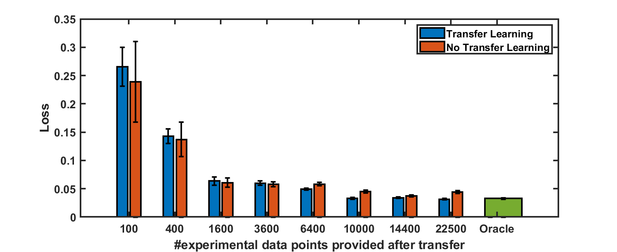
As can be seen in the blue bars of Figure 4, the greater the volume of real data coupled with transfer learning, the lower the loss, and the better the performance. This is to be expected, but this curve helps to give a better sense regarding how quickly we approach the limit of best-case performance, and suggests that the volume of real data used for oracle training could cut be cut down by nearly an order of magnitude while achieving comparable performance. One might argue that this is because the volume of real data used in this training is itself sufficient to effectively train this model; to that end, we consider the orange bars, which represent the loss of models trained for 2000 epochs exclusively on the given volume of real data. This, coupled with the blue bars, suggests that - across all volumes of data - it is, at the very least, more consistent to use transfer learning. Models trained for that duration on exclusively real data sampled from the small domain tended to overfit, and had a much higher variance as a result. As the volume of real data used for fine-tuning increased, the difference between the two regimes of transfer vs. non-transfer learning became more pronounced, and the benefits of transfer learning become more noticeable. Thus we conclude that we can use transfer learning to cut down on the quantity of real data needed, while sacrificing relatively little up to a ~75% cut of data requirements.

Experiment 2

Next, we wish to address the question of how structurally dissimilar a model can be while still making this transfer learning effective. To this end, we varied $n$ from our first experimental model, and generated data with our second experimental model. In each case, we performed a ~95% cut in the volume of real data relative to the volume of data used to train each oracle.

Figure 5: Bar plots of model loss as the model being learned is varied, as a means of representing increases in complexity or structure. As can be seen, within this range of complexity variation, transfer learning is consistently able to learn the system to a comparable degree across all cases.

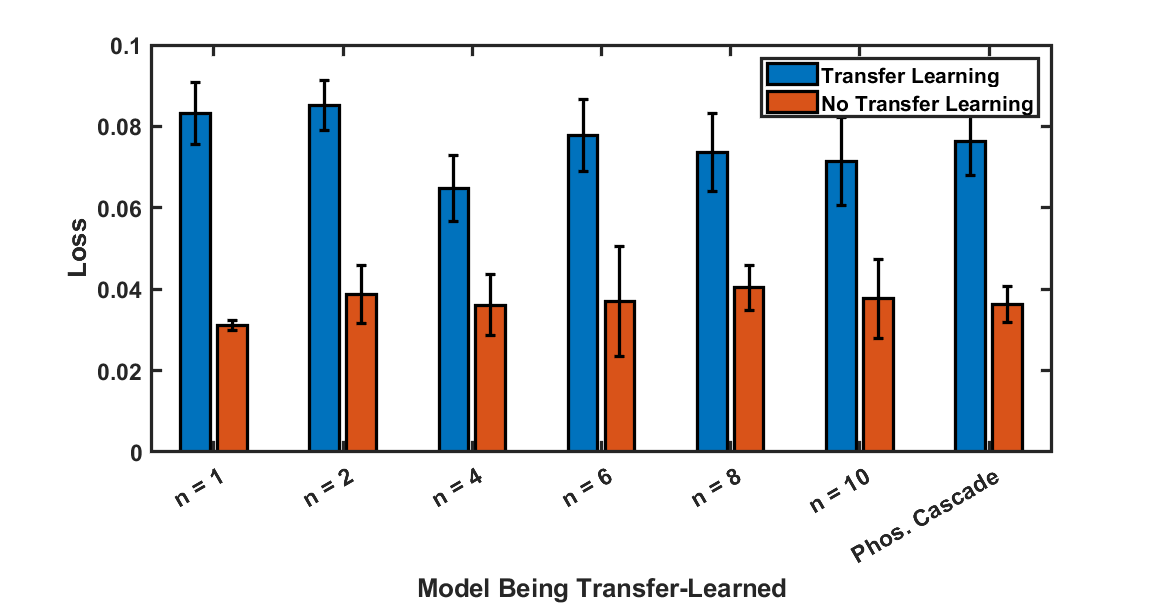
In Figure 5, we compare the loss of models trained with transfer learning to oracles for each - as can be seen, the transfer learning models performed consistently across all models being learned, and the oracles of each were similarly consistent. This suggests that the architectures of the models being learned are sufficiently similar that the transfer learning is effective, which is a promising sign for more applications in which the system being learned has been simplified significantly in its mathematical models.

Conclusion

Ultimately, we’ve developed a method by which to potentially reduce the volume of experimental data needed to effectively train a machine learning model by using synthetic data generated by a lower-complexity model of the system. We’ve demonstrated that it has the potential to cut down data requirements significantly while still achieving a high level of accuracy, and that the simple system used to generate data in the sense that the learning process can shore up some substantial structural differences betwen the simple and complex system. These findings are not necessarily limited strictly to synthetic biological learning tasks, either - any complex, data-starved phenomenon in which there is a simpler model to describe parts of the system may find value in this. Looking forward, one can consider deeper structural dissimilarities, as well as application with real synthetic biological data, rather than simply using two models of increasing complexity.