Applications of Deep Learning in Timbre Transfer

Exploring musical timbre transfer by leveraging prior art in differential digital signal processing (DDSP) and modern deep learning structures.

Introduction

Timbre is what distinguishes a flute from a trumpet, piano or any other musical instrument. Even if two performers play the same note, there is no ambiguity in the tone of their instruments. But unlike pitch (frequency) or amplitude (loudness), timbre is not a trivial metric; rather, it pertains much more to subjective qualities like raspiness, articulation and even musical intent. In this article, I’ll be discussing different data-driven approaches to extracting and manipulating this quality of sound using deep learning.

In particular I’d like to explore timbre transfer, where one instrument is made to sound like another while retaining most aspects of the original performance. I’ll be training an auto-encoder architecture first conditioned on the source instrument (whistling) then tuned to tracks of trumpets to achieve whistling-to-trumpet timbre transfer. Moreover, I’d like to reduce the complexity of previous architectures to achieve realtime results suitable for musical performance.

First, some context on sound and our perception thereof.

What is Sound?

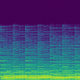
Our ears are sensitive to changes in air pressure over time, which we perceive as sound. Digital audio is analogous to this phenomenon, where its representation is a sequence of samples usually in the [-1, 1] range and discretized at a frequency high enough that it becomes indistinguishable from natural sources. This is known as the time domain, however all signals can be mapped to the frequency domain where the individual sinusoids that compose it are graphed against their respective amplitudes. Below is a Fourier transform applied to the sound of a trumpet from above:

It turns out that only the bottom-most frequency, \(f_0\), informs our ears of this note’s pitch. In fact, a pure sine wave at that frequency will sound similar to the trumpet.

The distinction between the trumpet and sine wave lies in the frequencies above \(f_0\), known as overtones. Moreover, certain musical instruments exhibit an interesting harmonic behavior where only the overtones that are multiples of \(f_0\) are actually prominent; this is the case for most instruments you could name, though some non-examples include the gong and timpani 2. Below is a spectrogram, which displays the frequency-domain of a signal over time. Observe the estimated \(f_0\) (implemented using the YIN algorithm ) and how its multiples (\(2 * f_0\), \(3 * f_0\), etc) evolve over time.

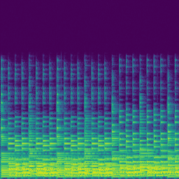
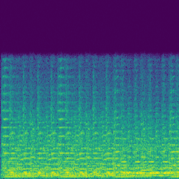
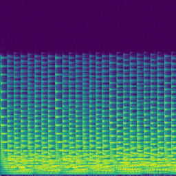
Try playing the audio clip above, whistle into the spectrogram or record your own instrument! The horizontal axis is time and vertical axis is frequency

So how do overtones relate to timbre? Well, the harmonic series is the most obvious distinguishing factor between different instruments playing the same pitch, so we could model timbre as the evolution of \(f_0\) and its overtones’ amplitudes over time. Note that this is assuming a strictly monophonic context (one note at a time), and overlooks non-harmonic parts of the signal (e.g. a flutist’s breathing). So this representation will still sound synthetic but it forms a good basis for what we’re trying to achieve.

Timbre Transfer

Perhaps the most obvious method for achieving timbre transfer is approximating the pitch of the source audio (as demonstrated above) and recreating it using a synthetic MIDI instrument. However, this discards much of the expressiveness which isn’t desireable in a musical performance.

Rather, data-driven approaches have shown promise in audio synthesis and existing deep learning architectures can be repurposed to achieve nuanced timbre transfer to various degrees of success. treats timbre transfer as an image-to-image problem, leveraging a Conditional Adversarial Networks architecture trained on natural images to transform spectrograms of audio signals. uses a Denoising Diffusion Implicit Model (DDIM) to achieve similar results. The audio is then synthesized from these spectrograms using the Inverse Fourier Transform or another neural network.

Keyboard	Guitar	String	Synth Lead

Images courtesy of

However, these methods rely on a dataset of audio tracks in two timbre domains, namely audio synthesized from MIDI instruments like in since recordings of performers will never match exactly. The results thereby sound synthetic; a better architecture would thus be self-supervised and trained on acoustic performances directly.

Proposed Model

I experimented with an auto-encoder architecture, where a network is trained to minimize the audible difference between some input audio track \(x\) and its re-synthesized counterpart \(\hat{x}\); so, the model attempts to recreate its input \(x\) by first encoding it to some latent representation \(z\) and decoding back to audio. Note that although over-fitting is possible, a one-to-one mapping (or, cheating) is impossible because \(z\) bottlenecks (has less dimensions than) \(x\). The appeal of this approach is that the problem is now self-supervised and can be trained directly on musical performances of the source instrument (e.g. whistling).

Next, the encoder is frozen (unaffected by gradient descent) and the decoder is trained anew on samples of the target instrument (e.g. trumpet). So, the networks knows how to encode the source instrument to some \(z\), and hopefully its decoder has adapted to map \(z\) onto the target instrument.

The decoder doesn’t output audio directly, nor does it generate a spectrogram like in . Rather, it controls parameters of a harmonic oscillator proposed by which follows the intuition of timbre as discussed prior; that is, the oscillator has parameters for its \(f_0\) and the amplitudes of each harmonic overtone. Leveraging this strong inductive bias should reduce the size of the neural network enough to be applicable to realtime performances.

The encoder architecture is taken from , whose original application is tracking pitch; I don’t track pitch explicitely, rather demonstrates that CNNs can extract meaningful data from audio directly in the time domain. The issue with working in the frequency domain is shown in , where we’d need a high sampling rate (and thus the network needs to be that much faster) for high frequencies or a long sampling window (which yields a network with more parameters) for low frequencies. Note that there is a nice compromise to these issues by windowing the inputs and outputs , which I’d like to try later.

Finally, the loss I’m using is multi-scale spectrogram loss proposed in , which computes the L1 loss of two audio tracks in the frequency-domain on both a linear and log scale.

Encoder

The architecture of my model is largely inspired by Magenta’s Differentiable Digital Signal Processing (DDSP) paper, where differentiable sound processors are introduced. Although modules like reverb and a finite-impulse response (FIR) filter are included, I’m only experimenting with its harmonic oscillator for simplicity. The architecture proposed by is also an auto-encoder, however its latent representation is built on two heuristics (pitch, amplitude) rather than the audio itself. Despite this, is able to achieve natural sounding instruments but its controls are limited in expression, much like MIDI inputs. Realtime Audio Variational autoEncoder (RAVE) builds upon this by encoding a multiband decomposition of the source audio, or a collection of Fourier transforms with varying amount of bins to overcome limitations of the Nyquist frequency and limited precision of discretization. A single Fourier transform operates on a linear scale, where its frequency bins scale from \(0\) to its Nyquist frequency. However, humans hear on a logarithmic scale (i.e. A4 is \(440 \text{Hz}\) but an octave above that is \(880 \text{Hz}\)) so the transform has a bias towards low frequencies. Multiband decomposition approaches this by shifting the frequency bins using different window sizes of audio and letting the network generalize over the complete frequency spectrum. However, although has shown some incredible results and claims to run in realtime, that is not the case in practice .

In my experiment, I leverage a Convolutional Representation for Pitch Estimation (CREPE) ; it is a CNN-based pitch estimator that operates directly on the time-domain of an audio signal and achieves state of the art results. Rather than using its output, like in , I use its latent representation and train the network to generalize over more characteristics of sound than just pitch.

Decoder

introduced the idea of using oscillators for audio synthesis as opposed to raw waveform modeling. demonstrates that their architecture benefits from this inductive bias and is able to be significantly reduced in size. I wanted to experiment with the encoder for the part, so the decoder of my model remains unchanged from the original paper (for the most part). It consists of several dense layers, ReLU activation functions and layer normalization. In between these is a Gated Recurrent Unit (GRU). The harmonic oscillator from cannot produce sinusoids out of phase (the instantaneous phase is accumulated at each time step) but presumably the network needs some time dependency to form an audio envelope.

Image courtesy of Tellef Kvifte

Dataset

I trained the target instrument auto-encoder on the URMP dataset , which consists of individual recordings of performers across a variety of instruments. Specifically, I wrote a dataloader that selects only trumpet solo tracks and randomly samples a 4 second clip from each of them. The audio is down-sampled to \(16\text{kHz}\) because the dataset doesn’t contain many frequencies above \(8\text{kHz}\) and the reduced dimensionality allows for training on my M2 MacBook Air with a batch size of 16!

I also created my own whistling dataset, sampled from MIT students with varying levels of proficiency. The audio clips are normalized, silence is cutout and altogether I have around 2 hours of data.

Loss

Like and , I focus on perceptual loss which approximates human hearing. So, comparing waveforms in the time-domain would not work because humans aren’t sensitive to changes in phase whereas the signal changes drastically. I extend upon the multi-scale spectrogram loss proposed by , which consists of taking the L1 norm of the two inputs’ spectrograms (so phase is discarded) in both the linear and log domain. Note that human hearing is logarithmic, but spectrograms are not. I experiment upon this by employing the log Mel spectrogram which is an even better approximation of human hearing and used by , and .

Results

I trained 500 epochs of 16 times 4 second samples on a single M2 MacBook Air with Metal acceleration, totaling around 10 hours. Unfortunately, the loss converged but the network was not able to generalize over abstract characteristics of sound as I’d hoped. Rather, it learned to represent sound as a mellow mix of harmonics instead of anything useful. I think future experiments should penalize silence (or close to it), and perhaps add skip connections from the inputs’ power (explicitely calculated) to the decoder. Moreover, the size of the encoder was drastically reduced (a few orders of magnitude less parameters in both width and depth) so it’s possible the latent representation did not contain much meaningful data.

Sample synthesized waveforms at epochs 0, 250, and 470 respectively (loud sounds warning!).