Graph neural networks v.s. transformers for geometric graphs
With the recent development of graph transformers, in this project we aim to compare their performance on a molecular task of protein-ligand binding affinity prediction against the performance of message passing graph neural networks.
Introduction
Machine learning on graphs is often approached with message passing graph neural network (GNN) models, where nodes in the graph are embedded with aggregated messages passed from neighboring nodes
Background and relevant work
Graph neural networks on molecules
Graphs are comprised of nodes and edges, and we can model any set of objects with a defined connectivity between them as a graph. For example, social networks are a set of people and the connectivity between them is defined by on who knows who. We can also see that grid data formats, like images, are also graphs where each pixel is a node and edges are defined to the adjacent pixels. Any sequential data, such as text, can be modeled as a graph of connected words. In this section we focus on graphs of molecules where nodes are atoms and edges are defined between atoms. These edges are often defined by the molecular bonds, or for atoms with 3D coordinate information the edges can be defined by a spatial cutoff $d$ based on the Euclidean distance between nodes. Given a graph we can use a graph neural network to learn a meaningful representation of the graph and use these representations for predictive tasks such as node-level prediction, edge-level prediction, or graph-level prediction. Graph neural networks learn through successive layers of message passing between nodes and their neighboring nodes.
An important property of many GNNs applied on 3D molecules is SE(3)-equivariance. This means that any transformation of the input in the SE(3) symmetry group–which includes all rigid body translations and rotations in $\mathbb{R}^3$ –will result in the same transformation applied to the output. This property is important for the modelling of physical systems; for example if the prediction task is the force applied on an atom in a molecule, rotation of the molecule should result in the model predicting the same forces but rotated. In some tasks we do not need equivariance but rather SE(3)-invariance (which is a subset of SE(3)-equivariance) where any transformation of the input in the SE(3) symmetry group results in the same output. This is often the case when the task of the model is to predict a global property of the molecule which should not change if all 3D coordinates of the molecule are translated and rotated. SE(3)-invariance will be required for our model of binding affinity as global rotations and translations of the protein-ligand structure should yield the same predicted binding affinity.
Early SE(3)-equivariant GNNs on point clouds used directional message passing
Graph transformers on molecules
With the proliferation of transformers in the broader field of machine learning, this has also led to the development of graph transformers. In a transformer model each node attends to all other nodes in the graph via attention where the query is a projection of the feature vector of a node, and the key and value is the projection of feature vectors of all other nodes. Hence, graph transformers and transformers applied to sequences (e.g. text) are largely similar in architecture. However, differences arise in the positional encodings in a graph transformer as it is defined in relation to other nodes in the graph
Motivation
Given the growing application of both GNNs and transformers we aim to compare their performance on the same task of protein-ligand binding affinity prediction. We also aim to compare models as we can see analogies between graph transformers and GNNs, where “message passing” in the graph transformer involves messages from all nodes rather than the local neighborhood of nodes. We view protein-ligand binding affinity prediction as a suitable task to compare the two architectures as there are aspects of both the GNN and graph transformer architecture that would be advantageous for the task: binding affinity is a global prediction task for which the graph transformer may better capture global dependencies, conversely binding affinity is also driven by local structural orientations between the protein and ligand which the GNN may learn more easily.
Problem definition
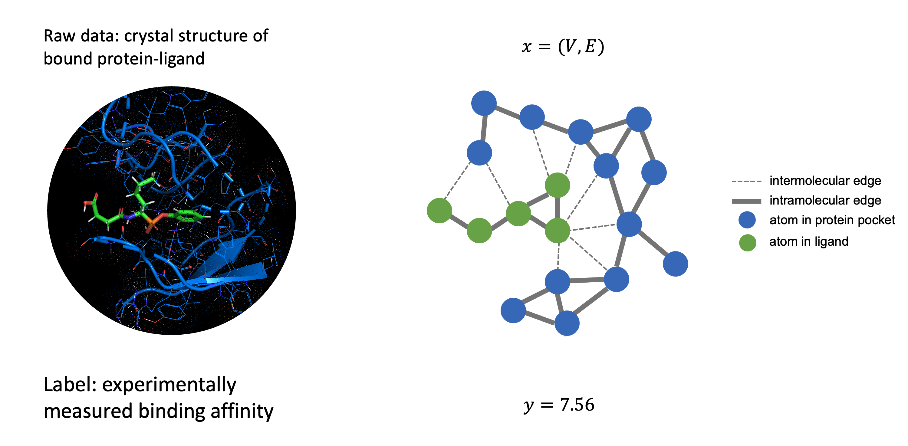
- The input to the model is a set of atoms for the protein pocket $X_{\mathrm{protein}}$ and ligand $X_{\mathrm{ligand}}$, for which we have the atomic identity and the 3D coordinates, and the binding affinity $y$ for the structure.
- For the graph neural network we define a molecular graph of the protein ligand structure $G=(V,E)$ where $V$ are the $n$ nodes that represent atoms in the molecule and the edges $E$ are defined between two nodes if their 3D distance is within a radial cutoff $r$. We further define two types of edges: intramolecular edges for edges between nodes within $X_{\mathrm{protein}}$ and $X_{\mathrm{ligand}}$, and intermolecular edges for nodes between $X_{\mathrm{protein}}$ and $X_{\mathrm{ligand}}$.
- For the graph transformer it is applied to the whole set of atoms $(X_{\mathrm{protein}}, X_{\mathrm{ligand}})$, and we can use the 3D coordinates of the atoms to derive positional encodings.
- Performance is determined by the root mean squared error, Pearson, and Spearman correlation coefficients between true binding affinity and predicted binding affinity.

Dataset
We use the PDBbind dataset for the protein-ligand structures and binding affinity. In addition, for benchmarking we use the benchmark from ATOM3D
Architecture
Graph neural network

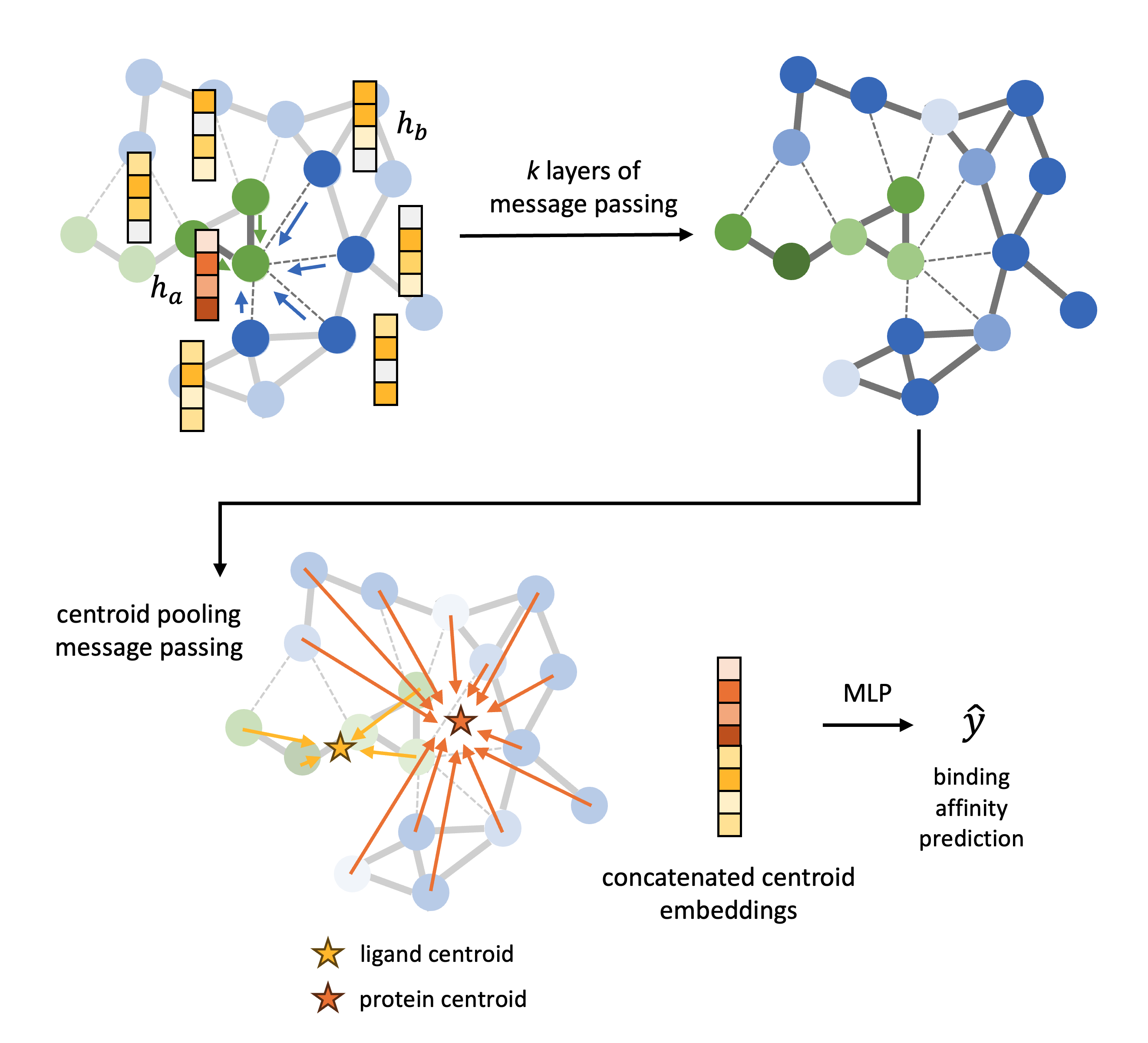
A graph is constructed from the atomic coordinates of the atoms in the protein pocket $X_{\mathrm{protein}}$ and ligand $X_{\mathrm{ligand}}$ where the nodes are the atoms. Intramolecular edges are defined between nodes within $X_{\mathrm{protein}}$ and $X_{\mathrm{ligand}}$ with a distance cutoff of 3 Å, and intermolecular edges for nodes between $X_{\mathrm{protein}}$ and $X_{\mathrm{ligand}}$ with a distance cutoff of 6 Å. The model architecture is defined as follows:
(1) Initial feature vectors of the nodes are based on a learnable embedding of their atomic elements. The edge features are an embedding of the Euclidean distance between the atomic coordinates. The distance is embedded with a Gaussian basis embedding which is projected with a 2 layer MLP.
(2) We define two types of messages in the GNN, given by the two types of edges, intermolecular messages and intramolecular messages. The architecture used for the two types are messages are the same but the weights are not shared, this is to reflect that information transferred between atoms within the same molecule is chemically different to information transferred between atoms of different molecules. The message passing equation uses the tensor product network introduced by e3nn

where node $b$ are the neighbors of node $a$ in $G$ given by intermolecular or intramolecular edges denoted with $t$. The message is computed with tensor products between the spherical harmonic projection with rotation order $\lambda = 2$ of the unit bond direction vector, \(Y^{(\lambda)}({\hat{r}}_{a b})\), and the irreps of the feature vector of the neighbor $h_b$. This is a weighted tensor product and the weights are given by a 2-layer MLP, $\Psi^{(t)}$ , based on the scalar ($\mathrm{0e}$) features of the nodes $h_a$ and $h_b$ and the edge features $e_{ab}$. Finally, $LN$ is layer norm. Overall, the feature vectors of the nodes are updated by intermolecular and intramolecular messages given by the tensor product of feature vectors of intermolecular and intramolecular neighbors and the vector of the neighbor to the node.
(3) After $k$ layers of message passing we perform pooling for the nodes of $X_{\mathrm{protein}}$ and the nodes of $X_{\mathrm{ligand}}$ by message passing to the “virtual nodes” defined by the centroid of the protein and ligand, using the same message passing framework outlined above.
(4) Finally, we concatenate the embedding of the centroid of the protein and ligand and pass this vector to a 3 layer MLP which outputs a singular scalar, the binding affinity prediction.
Graph transformer

The model architecture is as follows:
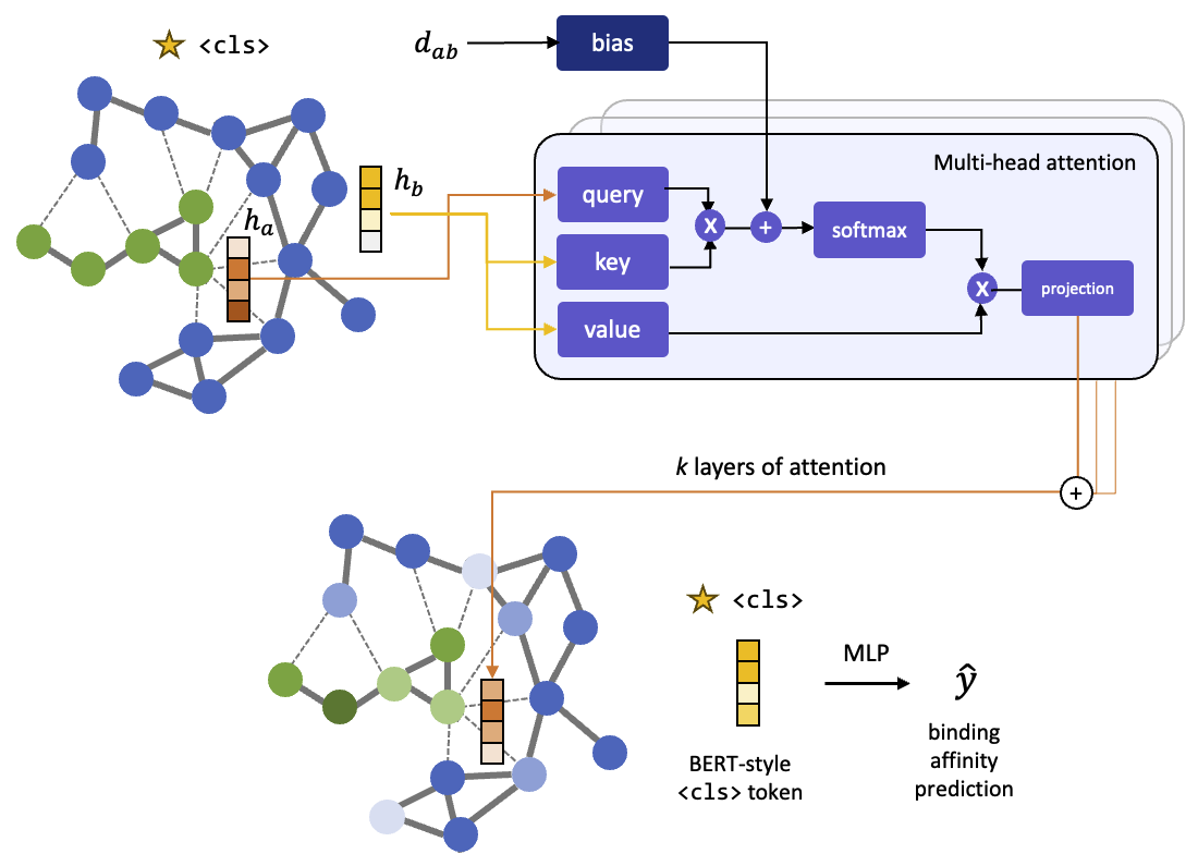
(1) Initial feature vectors of the nodes are based on a learnable embedding of their atomic elements.
(2) The graph transformer architecture is based on graphormer <cls> token used in the BERT model which functions as a virtual global node
(3) We take the final embedding of the <cls> node and pass it through a 3 layer MLP which outputs a singular scalar, the binding affinity prediction.
Loss function
Both models are trained to minimise the root mean squared error between the predicted binding affinity and true binding affinity.
Experiments
In order for the results to be comparable between the two models, both models have approximately 2.8 million parameters.
GNN model details:
- 2 layers of message passing, number of scalar features = 44, number of vector features = 16. Number of parameters: 2,878,011
- 4 layers of message passing, number of scalar features = 32, number of vector features = 13. Number of parameters: 2,767,269
- 6 layers of message passing, number of scalar features = 26, number of vector features = 12. Number of parameters: 2,764,431
We compare GNNs with different numbers of layers to compare performance across models which learn embeddings from various $k$-hop neighborhoods.
Graph transformer model details: 8 attention heads, 8 layers, hidden dimension = 192, feed forward neural network dimension = 512. Number of parameters: 2,801,155
Both models were trained for 4 hours on 1 GPU with a batch size of 16, Adam optimiser, and a learning rate of $1 \times 10^{-3}$. We show the results for the 30% and 60% sequence-based splits for the protein-ligand binding affinity benchmark in Table 1 and 2 respectively.
Table 1. Protein-ligand binding affinity task with 30% sequence based split. ProNet
| Model | Root mean squared error $\downarrow$ | Pearson correlation coefficient $\uparrow$ | Spearman correlation coefficient $\uparrow$ |
|---|---|---|---|
| ProNet | 1.463 | 0.551 | 0.551 |
| GNN 2 layer | 1.625 | 0.468 | 0.474 |
| GNN 4 layer | 1.529 | 0.488 | 0.477 |
| GNN 6 layer | 1.514 | 0.494 | 0.494 |
| Graph Transformer | 1.570 | 0.476 | 0.469 |
Table 2. Protein-ligand binding affinity task with 60% sequence based split. ProNet
| Model | Root mean squared error $\downarrow$ | Pearson correlation coefficient $\uparrow$ | Spearman correlation coefficient $\uparrow$ |
|---|---|---|---|
| ProNet | 1.343 | 0.765 | 0.761 |
| GNN 2 layer | 1.483 | 0.702 | 0.695 |
| GNN 4 layer | 1.471 | 0.717 | 0.719 |
| GNN 6 layer | 1.438 | 0.722 | 0.704 |
| Graph Transformer | 1.737 | 0.529 | 0.534 |
Discussion
GNNs perform better than graph transformers
From the benchmarking we can see that the graph transformer model performs worse than the GNNs for the 30% and 60% sequence split for protein-ligand binding affinity. An intuitive explanation for why graph transformers perform worse is it may be difficult for the graph transformer to learn the importance of local interactions for binding affinity prediction as it attends to all nodes in the network. Or in other words, because each update of the node involves seeing all nodes, it can be difficult to decipher which nodes are important and which nodes are not. In order to test if this is true, future experiments would involve a graph transformer with a sparse attention layer where the attention for nodes beyond a distance cutoff is 0. Converse to the lower performance of graph transformers, the results show that deeper GNNs which “see” a larger $k$-hop neighborhood perform better. However, we did not push this to the extreme of implementing a GNN with enough layers such that the $k$-hop neighborhood is the whole graph which would be most similar to a graph transformer as it attends to all nodes. This is because very deep GNNs are subject to issues like oversmoothing where all node features converge to the same value
The GNN may also perform better than the graph transformer due to the higher order geometric features used by the e3nn GNN message passing framework, compared to the graph transformer which only has relative distances. To further explore this future work will involve implementing the equiformer graph transformer
Depth v.s. width
Deeper GNNs (2 v.s. 4 v.s. 6 layers) with an approximately constant total number of parameters acheived better performance across both protein ligand binding affinity tasks. This was also observed in the image classification field with the development of AlexNet where deeper networks were shown to significantly improve performance
Model performance v.s. graph size
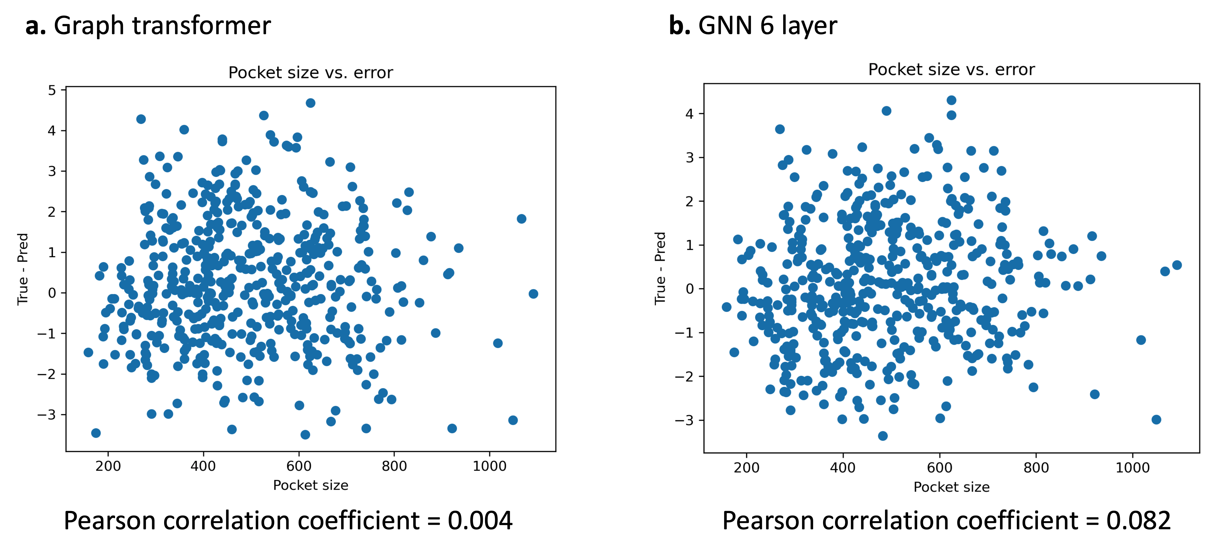
We compared the error of the prediction v.s. the number of atoms in the graph to test the hypothesis if larger graphs are more difficult to make predictions on. However, correlation between error and number of atoms in the graph all yielded very low pearson correlation coefficients ($< 0.1$) for all experiments (Figure 4). Thus, the number of atoms in the graph has minimal effect on the predictive ability of the model. This may suggest why the the graph transformer–which is able to attend to all nodes in the graph–did not perform much better as the GNN performance does not degrade significantly with larger graphs.

Future work
We implemented a relatively simplistic graph transformer in this project. While we concluded for this vanilla implementation of the graph transformer the GNN outperforms the graph transformer there are many more complex graph transformer architectures that we could explore to build more expressive architectures. In this section we explore some possible ideas.
Using cross-attention for better representation of protein-ligand interactions. In this project, we adapted the graph transformer from graphormer
Heirarchical pooling for better representation of amino acids. Graph transformer performance could also be lifted by defining better pooling strategies than using the <cls> token from a set of all atoms to predict binding affinity. In this project the graphs were defined based on the atoms in the graph. However, proteins are comprised of an alphabet of 21 amino acids. Thus, it may be easier for the model to learn more generalisable patterns to the test set if the model architecture reflected how proteins are comprised of animo acids which are comprised of atoms. This has been achieved in models using hierarchical pooling from the atom-level to the amino acid-level and finally to the graph-level
A hybrid approach: GNNs with Transformers. Finally, we could improve also performance further by taking a hybrid approach. That is, the GNN first learns local interactions followed by the graph transformer which learns global interactions and pools the node embeddings into a global binding affinity value. The motivation for this design is to leverage the advantages of both models. The GNN excels at learning local interactions while the graph transformer excels at learning global relationships from contextualised local interactions. This approach has been explored in other models for predicting drug-target interaction
Conclusion
In this project we present a direct comparison of graph transformers to GNNs for the task of predicing protein-ligand binding affinity. We show that GNNs perform better than vanilla graph transformers with the same number of model parameters across protein-ligand binding affinity benchmarks. This is likely due to the importance of capturing local interactions, which graph transformers may struggle to do. We also show that deeper GNNs perform better than wider GNNs for the same number of model parameters. Finally, future work in this area will involve a implementing more complex graph transformers, or taking a hybrid approach where we capture local interactions with a GNN and global interactions with a graph transformer.