Projected fast feedforward networks

Abstract

Introduction

Compression of neural networks is a crucial task in Machine Learning. There are three important performance metrics that we should take into account when deploying models:

Size of the model. Having a smaller number of parameters that describe the model makes transferring it over network faster. In addition, being able to concisely represent the differences between original and finetuned model would enable storing and distributing a lot of possible finetunings, such as in Stable Diffusion LORA
GPU memory needed to perform the inference. If the metric is lower, the model inference can be run on less expensive GPUs with less available memory. Some models could even be ran on smartphones or IoT devices
Inference time. We also can take into account how does the time scales with the size of the batch

Balancing these characteristics is a non-trivial task, since improvements in one of them could lead to a decline in other metrics. The optimal tradeoff depends on the environment in which the model is ran.

We will explore a way to significantly reduce the model size and the memory needed for inference, keeping the inference time reasonable. We achieve the size reduction by utilizing a common property of having small intrinsic dimension of objetive landscape that many models have.

There are several ways how the size of the model can be reduced. One of the popular techniques is model quantization. Quantization of a machine learning model involves decreasing the precision of weights for the sake of reduction of the total memory needed to store them. Quantized models can utilize 16, 8, or even 4-bit floats, with carefully selected summation and multiplication tables. There are different ways of dealing with the inevitable degradation of accuracy due to lack of precision, one possible way is described in paper

Another direction of model size optimization utilizes the notion of matrix low-rank approximation. The layers of neural networks are commonly represented as matrices, the simpliest example being the parameters of feedforward linear layer. Each matrix $A$ has a Singular Value Decomposition $A = U\Sigma V^*$, and, using this decomposition, it’s possible to get close low-rank approximation of $A$. We note that a matrix of size $n \times m$ of rank $k$ can be stored in $O((n+m)k)$ memory if we express it as a sum of outer products of $k$ pairs of vectors, so if $k$ is small, this representation uses much less memory than $O(nm)$ — the memory used by the dense representation. One of the papers that compresses models with low-rank approximation is .

However, we are going to explore another compression method, which utilizes small dimensionality of optimization landscape, which is common for many model-task pairs. When training a neural network, we have some loss $\mathcal{L}$, and a parameter space $\mathbb{R}^{p}$. Then, we are trying to find $v \in \mathbb{R}^{p}$ such that $\mathcal{L}(v)$ is minimized. Instead of searching over the whole space, we generate a linear operator $\phi\colon \; \mathbb{R}^{d} \to \mathbb{R}^{p}$, where $d < p$, and parametrize $v$ as $v = \phi u$, where $u \in \mathbb{R}^{d}$. Li et al. found that if the the matrix of $\phi$ has normalized columns, for many tasks it’s possible to find a network, parametrized the way above, where $d$ is significantly smaller than $p$, such that the network has at least 90% of metric value of the original network. Then, if our way to generate random projection matrix is seeded deterministically, we only need to store $d$ floats, which are the coefficients of $u$. During inference, we re-create $\phi$, and restore the parameters of original architecture $v = \phi u$. The compression ratio of this method is $\frac{p}{d}$. In this blog, we will explore its potential modifications, and evaluate them by running experiments.

Basic experiment

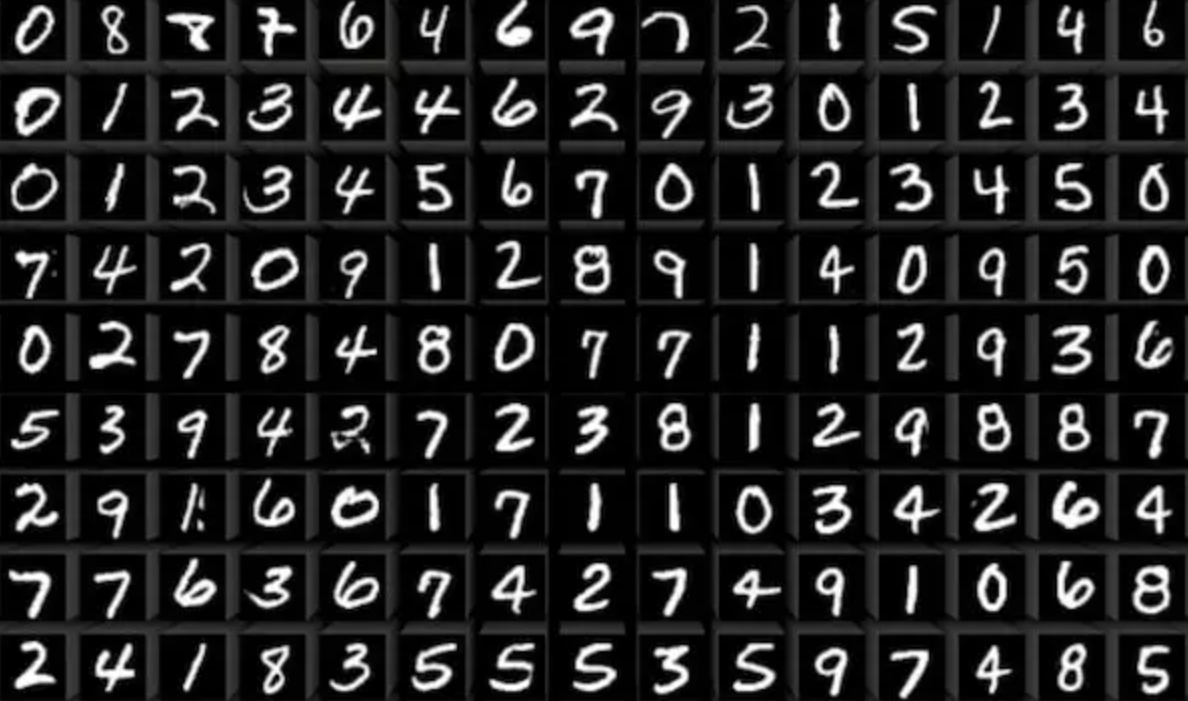
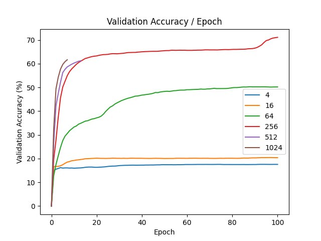
First, we test the method without any modifications. We use dataset MNIST , containing 30000 $28 \times 28$ monochrome images of digits. Each image belongs to one of 10 classes, depending on the digit, and the task of the model is to classify these digits.

For each of the experiment, we use a neural network with one hidden layer with 128 units and ReLU activations. We optimize the parameters with Adam and learning rate $10^{-4}$. The training is ran for $100$ epochs, our batch size is $128$.

d	final val acc
4	17.56
16	20.39
64	50.2
256	71.1
512	61.25
1024	61.66
original	95.65

Better initialization

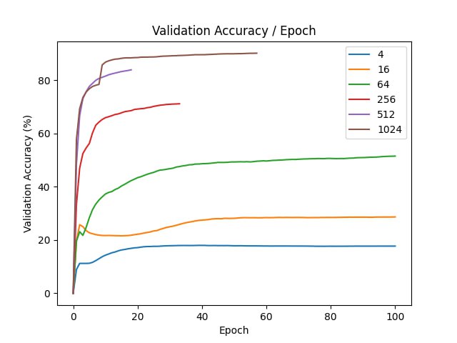
We’ve noticed that the optimization of the compressed model does not converge fast. To initialize better, we can use pre-trained weights of non-compressed model $v$.

Let $A$ be the projection matrix that we used in the compression. Then, to convert compressed parameters of a model to the original ones, we need to multiply by $A$ on the left. The idea is to start from the compressed parameters, such that after going to uncompressed space, they would be as close to $v$ as possible by Eucledian distance. Then, we can use the formula for projection onto a linear subspace:

\[u^{*} = \mathop{argmin}_u ||Au - v||^2 \Rightarrow u^{*} = (A^TA)^{-1}A^Tv\]

By initializing $u$ this way, we achieve a faster convergence of the optimizer, because after projecting to subspace and returning to original coordinates, we get a parameter vector that is close to the optimal one, so it should be near the optimum in the coordinates of projection.

In our experiments, we compare how fast does the model train with random initializtion and with projection initialization.

d	final val acc
4	17.72
16	28.68
64	51.52
256	71.18
512	83.93
1024	90.18
original	95.65

Distillation

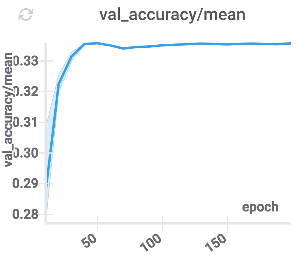
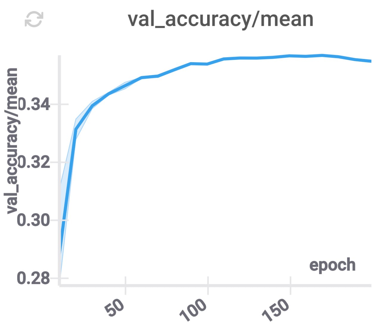
The concept of model distillation was introduced by . The main idea is to train a compact model (“student”) to emulate a larger, pre-trained model (“teacher”). In our case, the compact model would be a reparametrized model with $d$ dimensions, while the “teacher” model has all the original parameters. When training, we regress the mean square difference between the logits of the original and compact model.

We initialize the compressed model with the projection of the original model as in the previous section. In our experiments, we’ve noticed that this training procedure has comparable convergence speed, however, its validation accuracy reaches a plateau on a lower value than in regular training procedure.

CIFAR-10 experiment. Network is logistic regression. Projections for d=700, on the left: with distilation, on the right: without distilation

Independent projections for layers

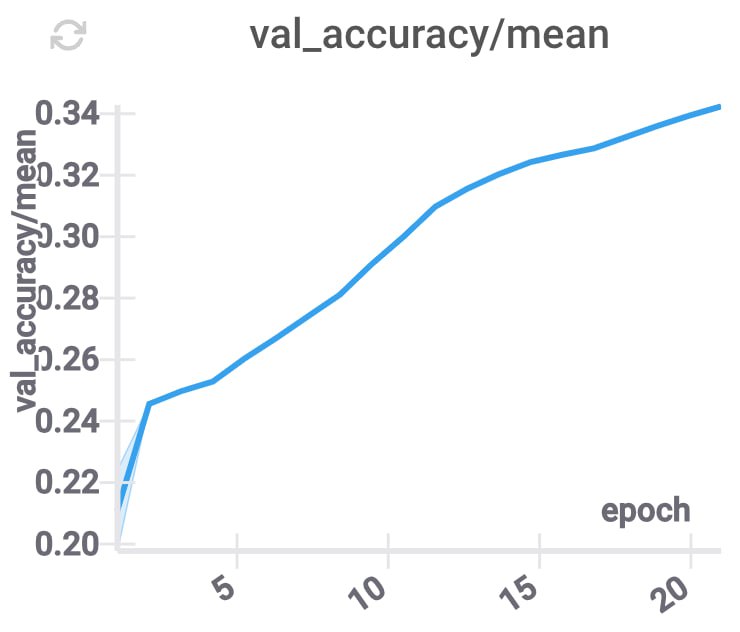
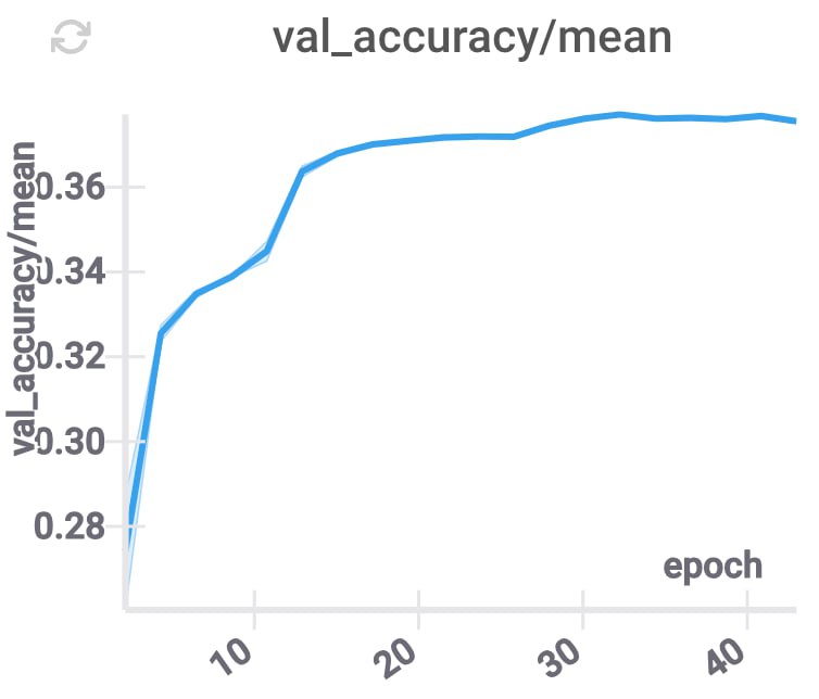
In many cases, the model we are compressing contains several independent layers. Therefore, we can try to split the coordinates in the space to which we are projecting parameters so that each coordinate corresponds to exactly one layer. This constraint corresponds to the matrix of $\phi$ being block-diagonal.

These changes improve the accuracy, and decrease the inference time (because for each layer we only need to use some part of the compressed coordinates), while keeping $d$ constant.

CIFAR-10 experiment. Network has one hidden layer with 32 units. On the left: one projection for d=2500. On the right: separate projections with d=500 and d=100

GPU memory utilization

Let we want to make inference with minimal possible usage of RAM. Let’s assume that the architecture of model that we are evaluating is an MLP. Then, using the compressed representation, we can use no more than $O(\max(d, L))$, where $d$ is the dimension to which we compressed the model, and $L$ is the maximum size of the layer.

We describe the inference prodcedure consuming this little memory. We need to sequentially apply each of the feedforward networks in our MLP. For each layer, we have to transform the input vector $x$ to the output $y$. We fill in the output vector with zeros, and for each index $(i, j)$ in the weight matrix we need to make an update $y_i \leftarrow y_i + A_{ij}x_j$. However, we don’t store any of the parameters in memory except for $d$ compressed parameters. So, in order to get the value of $A_{ij}$, we need to take the dot product of a row in the projection matrix and a vector of compressed parameters.

It is not obvious how to random access a row in a random matrix, where all columns should be normalized, and the outcomes during train and inference are consistent. We note that the true randomness of the projection matrix is not important for us. So, instead we can generate the $i$-th row by seeding the random to $i$ and generating a row. During train, we generate the whole matrix this way, and compute the normalization coefficients of columns, which are included into the model’s representation in memory. During inference, to get the $i$-th row, we just need to sample a row and divide it by normalization coefficients pointwise. We have checked that this way of generating the projection matrix has no negative effects on the performance of the compressed model, compared to the truly random option.

Diffusion models

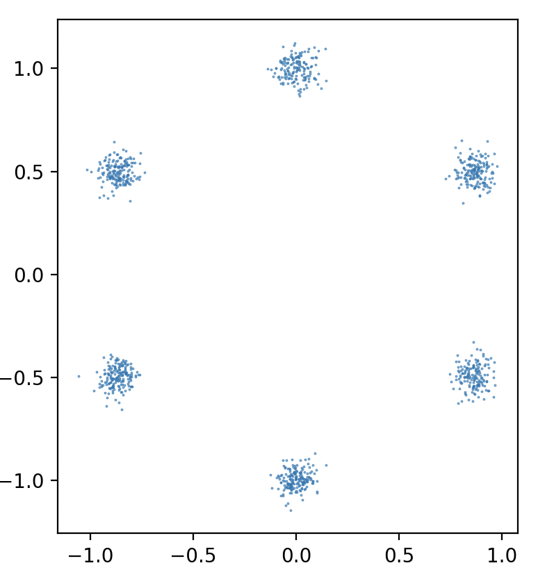
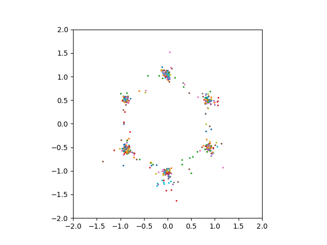
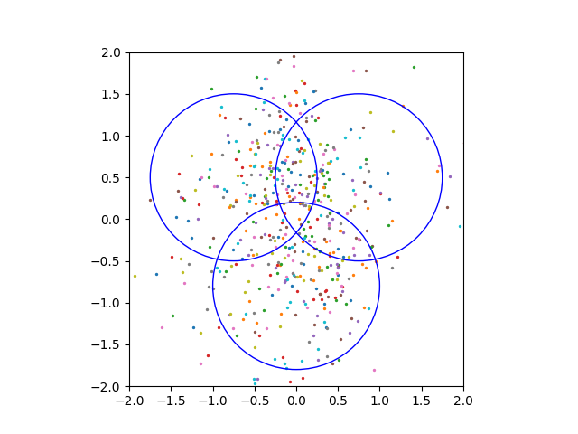
We have also attempted to apply model compression to a different domains besides image classification. One of the problems we considered is generating 2D points from a certain distribution using a diffusion model. In this setup, we have a neural network that predicts the noise for a pair $(x, t)$ — point in space and time.

We use continuous time on $[0, 1]$, linear noise schedule with $\beta_{min} = 0.3$, $\beta_{max} = 30$, various-preserving SDE, batch size $64$, sampling timesteps $100$, ODE sampler. The distribution that we are trying to learn is a mixture of $6$ gaussians. We use an MLP score net with $2$-dimensional input and $32$-dimensional Gaussian Fourier Projection time embeddings.

However, even setting the compression dimension $1000$ or $5000$ did not enable us to see good sampling results.

On the left: sampling result with original model. On the right: sampling with compressed model, d=1000

Conclusion

We have discussed a way to compress models, decreasing its size by several orders of magnitude. We identified ways to improve the validation accuracy of compressed models, such as doing the initializtion with projection and having independent projections for layers. This technique leads to surprising consequences, such as being able to do machine learning model inference with very small amount of RAM.