Neural PDEs for learning local dynamics and longer temporal rollouts

6.S898 deep learning project

Partial differential equations

At the continuum level, spatiotemporal physical phenomena such as reaction-diffusion processes and wave propagations can be described by partial differential equations (PDEs). By modeling PDEs, we can understand the complex dynamics of and relationships between parameters across space and time. However, PDEs usually do not have analytical solutions and are often solved numerically using methods such as the finite difference, finite volume, and finite element methods . For example, the finite element method (FEM) approximates PDE solutions by first discretizing a sample domain into a mesh of interconnected elements and then solving a system of equations iteratively given a set of boundary conditions, initial conditions, and material properties.

In this blog, we will show two examples of PDEs, one of which is the Navier-Stokes equation which describes the dynamics of viscous fluids. The equation below shows the 2D Navier-Stokes equation for a viscous and incompressible fluid in vorticity form on a unit torus, where \(w\) is the vorticity, \(u\) the velocity field, \(\nu\) the viscosity coefficient, and \(f(x)\) is the forcing function. The solution data were from the original paper where the problem, with a periodic boundary condition, was solved with a pseudospectral method using a 1e-4 time step with the Crank-Nicolson scheme.

\[\begin{gather} \partial_t w(x, t) + u(x, t) \cdot \nabla w(x, t) = \nu \Delta w(x, t) + f(x), \quad x \in (0,1)^2, t \in [0,T] \\ \nabla \cdot u(x, t) = 0, \quad x \in (0,1)^2, t \in [0,T] \\ w(x, 0) = w_0(x), \quad x \in (0,1)^2 \end{gather}\]

We can visualize the 2D PDE solution over the 50 time steps:

Solution of 2D Navier-Stokes PDE - drag the slider!

Motivations for neural PDEs

Well-established numerical methods are very successful in calculating the solutions of PDEs, however, these methods require high computational costs especially for high spatial and temporal resolutions. Furthermore, it is important to have fast and accurate surrogate models that would target problems that require uncertainty quanitifcation, inverse design, and PDE-constrained optimizations. In recent years, there have been growing interests in neural PDE models that act as a surrogate PDE solver, especially neural operators that aim to learn the mapping between input and output solution functions. These models are trained on numerical solutions from existing methods and inferences are orders of magnitude faster than calculating the solutions again through numerical methods.

In this article, I will first examine if we can apply neural networks to learn the dynamics in PDE solutions and therefore replace PDE solvers with a neural PDE as the surrogate solver. We will start with a base U-Net model with convolutional layers. Next, I will examine the neural operator methods, notably the Fourier Neural Operator (FNO). Primarily, the Fourier neural operator has proven to predict well for PDE solutions and we will use it to compare with the U-Net model on the representations learnt in the Fourier layers. Next, I will examine the FNO’s performance on another PDE with two dependent states. We will notice that the FNO is capable of learning lower frequency modes but fail to learn local dynamics and higher frequency modes. We then finally introduce some improvements to the FNO to tackle this problem involving local dynamics and long term rollout errors.

Dataset and training schemes for the 2D Navier-Stokes PDE

For the dataset, I will start with the 2D time-dependent Navier-Stokes solution (\(\nu\) = 1e-3) that was shipped from Zongyi Li et al’s paper . The problem for any given model would then be to learn the mapping from an input solution (vorticity) of t=[0,10] to the solution of t=(10, 40]. For all models involving Navier-Stokes, the original implementations were used, but implementations were improved or new ones were added for the second PDE problem which more details will be shared in later parts of the article. We use 1000 solutions for training and 200 for the test dataset. The models are trained with 500 epochs with an initial learning rate of 0.001, the AdamW optimizer is used with a cosine annealing scheduler. Unless otherwise specified, a relative L2 loss is used for training and prediction of each data batch. For U-Net and FNO2D, the models use 2D convolutions in the spatial domain and recurrently predict through the time domain (autoregressive training). For FNO3D, the time domain is included as the 3rd dimension in the input data for the FNO to learn both spatial and temporal dependencies within the solutions.

Base model (U-Net)

Let’s begin with examining whether a U-Net with convolutional layers can be used to learn the dynamics. U-Net is a popular model architecture for image to image predictions and image segmentation tasks. It consists of a series of downsampling and upsampling layers with skip connections, and my re-implementation is based on this repo.

We can use the U-Net to learn the features from the input PDE solution frames and predict the solution in the next time step, treating the 2D solution as an image. As for the time component, the surrogate model takes the input solution from the previous k time steps to predict solution in the next k+1 time step. Then, the solution from the previous k-1 steps are concatenated with the predicted solution as the input back into the model to predict the next step, and so on. In a nutshell, the model is trained to predict autoregressively.

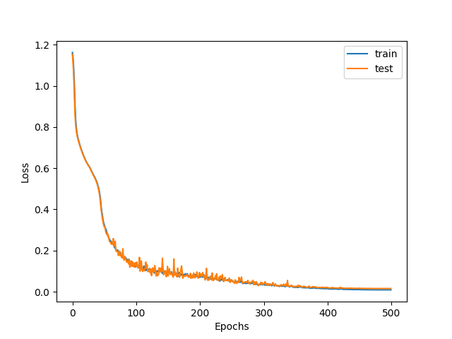
Training curve for U-Net with average relative L2 train and test loss

U-Net's prediction of 2D Navier-Stokes for unseen test set (id=42)

The U-Net seems to predict well for the 2D Navier-Stokes test set. However, the average final test loss of 0.0153 is still considerably high. For longer time rollout, the errors can accumulate. Let’s examine the FNO2d-t and FNO3d models next.

Fourier Neural Operators

Fourier neural operators (FNOs) try to learn the mapping between input functions and solution functions , for example, mapping the solutions from earlier to later time steps for time-dependent PDEs.

The authors introduced the Fourier layer (SpectralConv2d for FNO2d) which functions as a convolution operator in the Fourier space, and complex weights are optimized in these layers. The input functions are transformed to the frequency domain by performing fast Fourier transforms (torch.fft) and the output functions are then inverse transformed back to the physical space before they are passed through nonlinear activation functions (GeLU) to learn nonlinearity. Fourier transformations are widely used in scientific and engineering applications, such as in signal processing and filtering, where a signal / function is decomposed into its constituent frequencies. In the FNO, the number of Fourier modes is a hyperparameter of the model - the Fourier series up till the Fourier modes are kept (i.e. lower frequency modes are learnt) while higher frequency modes are truncated away. Notably, since the operator kernels are trained in the frequency domain, the model is theoretically capable of predicting solutions that are resolution-invariant.

Applying FNO2D and FNO3D on 2D Navier-Stokes time-dependent PDE

We reimplement and train the FNO2D model on the same train-test data splits for the 2D Navier-Stokes solution. Notably, the final average relative L2 loss (for test set) is 0.00602 after 500 epochs of training. Comparing this with the U-Net that is also trained and predicted with the same scheme, the FNO2D has an improved performance!

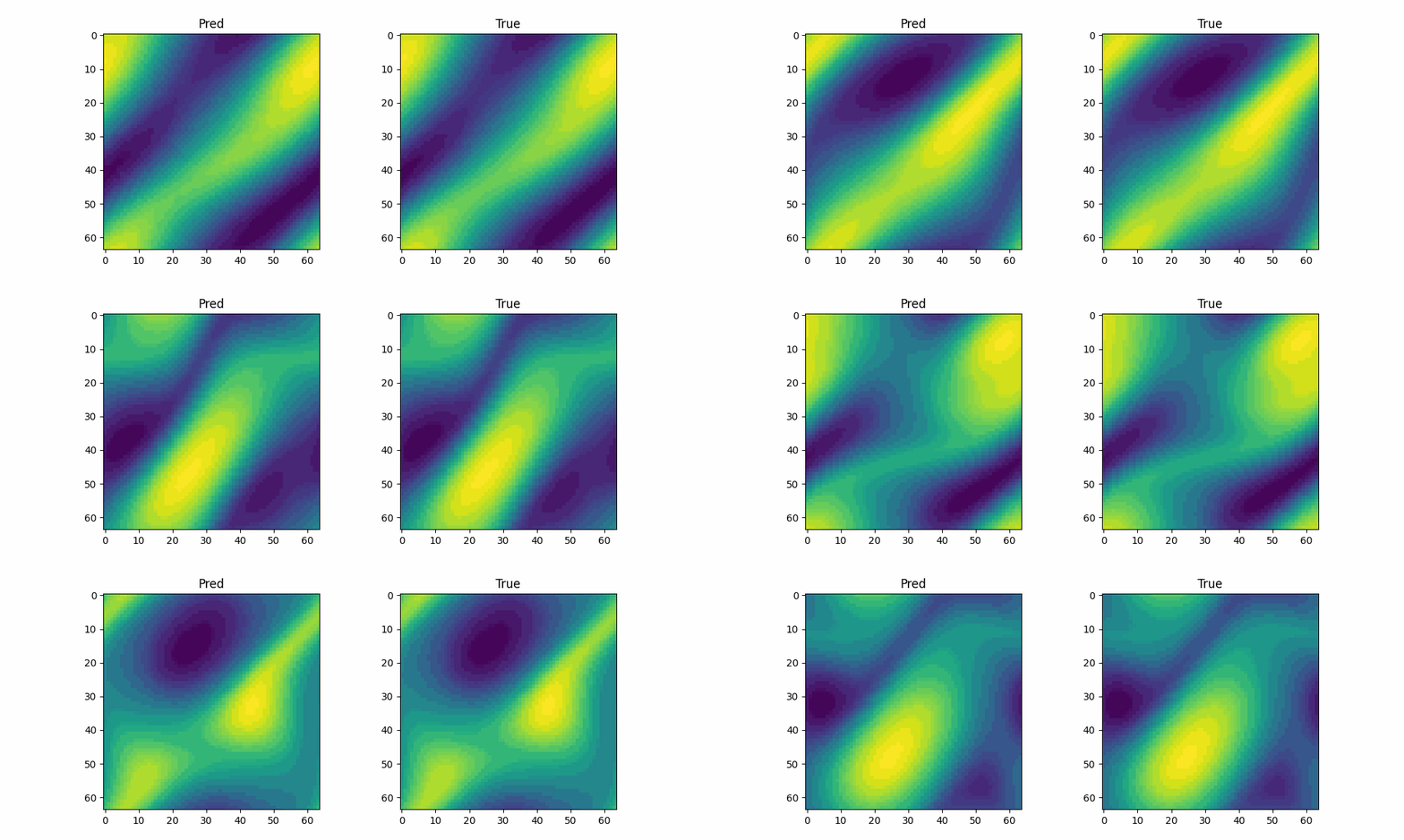
FNO2D's prediction of 2D Navier-Stokes for unseen test set (id=42)

The predicted solutions look impressive and it seems like the dynamics of the multiscale system are learnt well, particularly the global dynamics. Likewise, the FNO3D gives similar results. Instead of just convolutions over the 2D spatial domains, the time-domain is taken in for convolutions in the Fourier space as well. According to the authors, they find that the FNO3D gives better performance than the FNO2D for time-dependent PDEs. However, it uses way more parameters (6560681) compared to FNO2D (928661 parameters) - perhaps the FNO2D with recurrent time is sufficient for most problems.

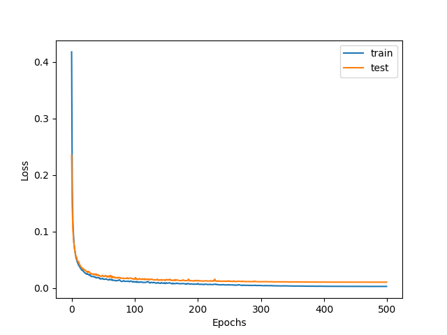
Training curve for FNO3D with average relative L2 train and test loss

FNO3D's prediction of 2D Navier-Stokes for unseen test set (id=42)

Representation learning in the Fourier layers

You might be curious how the Fourier layers learn the Navier-Stokes dynamics - let’s examine some weights in the SpectralConv3d layers (for the FNO3D). We take the magnitudes of the complex weights from a slice of each layer (4 Fourier layers were in the model).

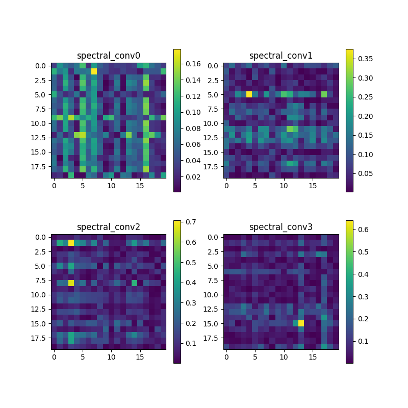
Visualizing weights in the Fourier layers

There seems to be some global features that are learnt in these weights. By learning in the Fourier space, the Fourier layers capture sinusoidal functions that can generalise better for dynamics according to the dynamical system’s decomposed frequency modes. For CNNs, we know that the convolutions in spatial domain would lead to the learning of more local features (such as edges of different shapes), as compared to more global features learnt in Fourier layers.

On the importance of positional embeddings

In FNO implementations, besides the input data for the 2D + time domains, the authors also append positional encodings for both x and y dimensions so the model knows the location of each point in the 2D grid. The concatenated data (shape = (B, x, y, 12)) is then passed through the Fourier layers and so on (note: B is the batch size, x and y the spatial sizes, and 12 consists of 10 t steps and 2 channels for positional encodings along x and y). It is important to understand that the positional embedding is very important to the model performance.

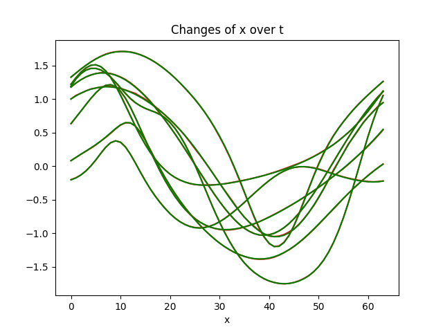
Original with positional encoding

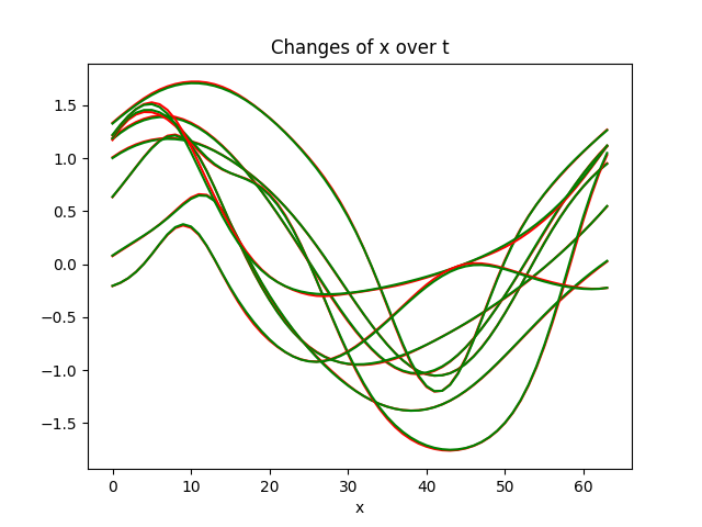
No positional encoding

We train the same FNO3D on the same data but this time without the positional encodings concatenated as the input. Simply removing these positional encodings for x and y domains cause the model to underperform. Here, we are comparing between FNO3D with and without positional encoding. FNO3D has a final relative test loss of 0.0106 but the test loss is 0.0167 without positional encodings. Inspecting the change of x over t for a sample test dataset, it then becomes more visible the differences in performances. Note that we also observe the data have well-defined sinusoidal functions in the dynamics.

Improving accuracies in predicting local dynamics and long-term rollouts in time-dependent PDEs

Let’s apply the FNO to other PDEs, particularly problems where local dynamics and long-term accuracies are important. Here, I introduce another PDE as an example - a coupled reaction heat-diffusion PDE with two dependent states.

\[\begin{gather} \kappa \frac{\partial^2 T}{\partial x^2} + \rho H_r \frac{\partial \alpha}{\partial t} = \rho C_p \frac{\partial T}{\partial t} \\ \frac{\partial \alpha}{\partial t} = A \exp \left( -\frac{E}{RT} \right) f(\alpha) \end{gather}\]

Based on the initial conditions of temperature (T) and degree of cure (alpha) and with Dirichlet boundary conditions on one end of the sample, the T and alpha propagate across the domain (here, the 1D case is examined). For certain material parameters and when initial conditions of T and alpha are varied, we can see that the dynamics can become chaotic after some time - we can visualize it below.

Solution of the above coupled PDE with 2 dependent states, solved using FEM. Drag the slider!

For this dataset, we aim to use the first 10 time steps of the solution (heat diffusion from x=0) as input to a neural PDE to predict the next N time steps of the solution. With 10 steps, we predict the 11th step and the prediction is concatenated with the last 9 steps to predict the next time step and so on. We first generate the training data by solving the PDE numerically using the Finite Element Method using the FEniCS package. Specifically, we use mixed finite elements with the continuous Galerkin scheme and a nonlinear solver with an algebraic multigrid preconditioner.

We use 1228 solutions for the training set and 308 solutions for the test set. The datasets are split into pairs of 10 trajectories, whereby the input data consists the solution of 10 time steps and the output data (to be predicted) consists the solution of the next 10 time steps. Since the neural PDE is trained to predict 10 to 1 time step, every batch is trained autoregressively and an L2 loss is taken for all 10 forward predictions before the sum is backpropagated in every batch. Likewise, the AdamW optimizer is used with an initial learning rate of 1e-4 and a cosine annealing scheduler. The models are trained for 300 epochs with a batch size of 16.

I initially tried the FNO1D implementation on my PDE dataset and notice that the errors accummulate with longer time rollouts using the trained model. FNO1D is used since we only have 1 spatial dimension in the 1D solution and the solutions are predicted recurrently, just like the use of FNO2D for the 2D Navier-Stokes example earlier. The FNO2D model was also used to convolve over both x and t. Both performances are not ideal within 1 cycle of forward prediction.

RevIN and other training tricks to improve accuracies in longer temporal rollout

To overcome this problem, there have been attempts to generally improve the accuracies of neural PDE models and also training tricks proposed to improve long-term accuracies in rollout. Using the FNO1D, I first tested out some training tricks, such as the pushforward and temporal bundling which are covered in the paper on message passing neural PDEs. Incorporating the reversible instance normalization layer (RevIN) gives a more promising improvement. With ReVIN, the input solution is passed through the normalizing RevIN layer before the FNO1d and the output solution is denormalized through the RevIN layer. Some examples of these tricks for longer term robust forecasting are covered in this repo.

Using a trained FNO1D with a RevIN layer, here is its prediction on an unseen test set starting from the first 10 time steps as the input solution. The true solution is used to predict up till 50 more time steps forward (5 full cycles forward). While the temperature is predicted with decent accuracies for first cycle (10 steps forward until t=60 shown), the errors accumulate over more steps.

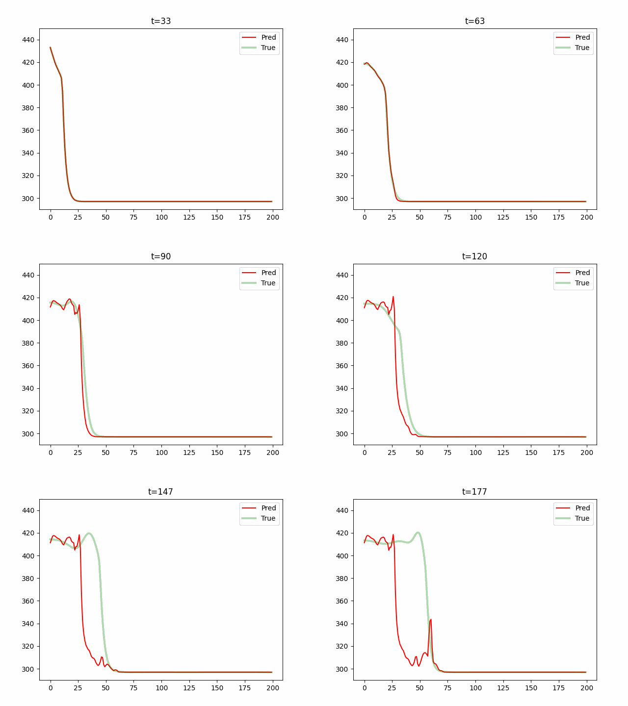
FNO1d's prediction (1)

Generally, we attribute this to the fact that the Fourier layers may not be able to learn more local changes in the dynamics since the higher frequency modes in the Fourier series are truncated away. The global dynamics of the propagating front (heat diffusion along x) are captured reasonably well (the positional encodings probably also have a large part to play). We want to build on the FNO to improve predictions for longer temporal rollout especially for multiscale dynamical systems with both global and local changes. Ideally, we want to take an input of a few time steps from a more expensive numerical solver and pass it through a trained surrogate model to predict N time steps (with N being as high as possible).

Introducing Large Kernel Attention

To overcome the problems highlighted for this PDE, we attempt to include a large kernel attention layer (LKA) that was introduced in the Visual Attention Network paper by Meng-Hao Guo et. al. The large kernel attention was first introduced as an alternative to the Vision Transformers (ViT) to enable higher spatial adapativity and long-range correlations. While simple to implement, the authors’ Visual Attention Network surpasses ViTs and CNNs on tasks such as object detection and pose estimation. A similar strategy was introduced last month for 2D problems although their implementation was not shared.

Therefore, it may be feasible to introduce attention mechanisms to learn local dynamics in PDEs better, and this can complement the Fourier layers which capture global dynamics better. Herein, we add the LKA layers after the Fourier blocks for the FNO1D, and the new model has 5056 more parameters (583425 to 588481). The performance is found to have greatly improved, especially for local dynamics in the unstable propagations.

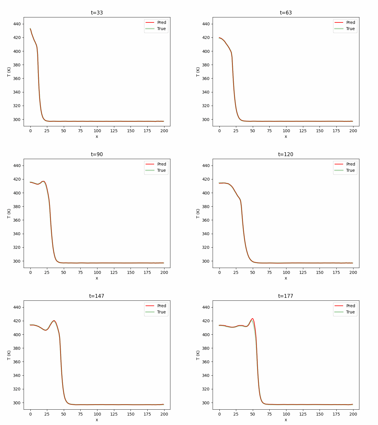
FNO1d + LKA's prediction (1)

For the same data, the addition of LKA gave improved accuracies over predictions in the next 50 time steps. We attribute this to the large kernel attention’s ability to focus on local dynamics at specific parts of the spatiotemporal changes. The LKA has 3 components: a spatial depth-wise convolution, a spatial depth-wise dilation long-range convolution, and a channel convolution.

\[\begin{gather} \text{Attention} = \text{Conv}_{1 \times 1}(\text{DW-D-Conv}(\text{DW-Conv}(F))) \\ \text{Output} = \text{Attention} \otimes F \end{gather}\]

I adapted from the LKA’s original implementation to apply to our 1D PDE. Let’s examine the predictions on another test data.

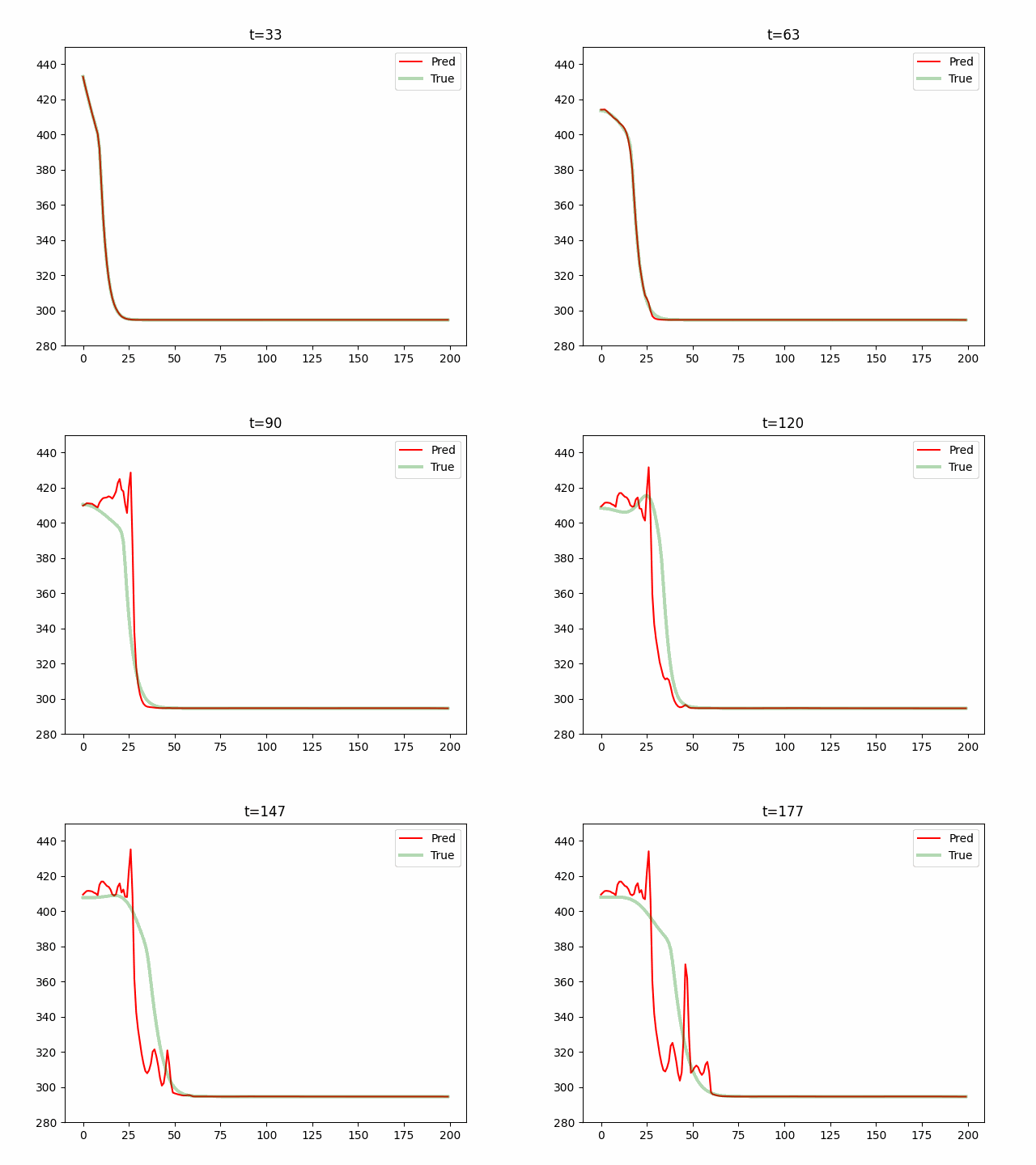
FNO1d's prediction (2)

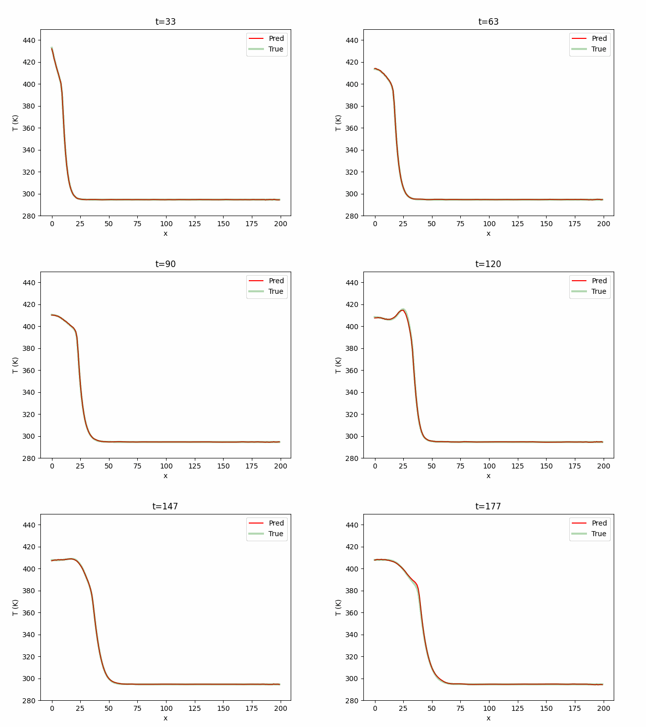
FNO1d + LKA's prediction (2)

While the predictions are significantly improved, the errors still accumulate with longer rollouts and the model fails to capture dynamics if we extend predictions till 100 steps forward. More work is needed to improve existing neural PDE methods before they can be used as foundational models for PDEs.

Conclusion

In this article, we have introduced the use of neural networks as potential surrogate model solvers for partial differential equations that can be expensive to solve using numerical methods. Compared to the base model U-Net, Fourier neural operators have introduced a novel and useful way of learning PDE solutions through convolutions in the frequency space. We first reimplemented the FNO2D and FNO3D on the 2D Navier-Stokes PDE solution shipped with their paper. While it achieves great performance learning global dynamics, existing models struggle to capture local dynamics (higher frequency modes are truncated away) and longer temporal rollouts. We demonstrate that despite adding a RevIN layer and several temporal training tricks, the FNO1D could not predict accurately the solutions of a coupled time-dependent PDE. With the inclusion of attention mechanism through the large kernel attention, the FNO1D’s performance significantly improved. We learn that introducing spatial attention can be useful and more work will be explored to improve predictions of multiscale spatiotemporal dynamical systems.