Cross-Lingual Fine-Tuning for Multilingual Text Embeddings
Exploring contrastively training text embeddings, and presenting a scalable, cheap and data-efficient method to train multilingual embedding models
Introduction
Recently, embeddings models have become incredibly popular as LLMs become more integrated into tools and applications. Embeddings models (specifically, Siamese encoder-only Transformers) are the state-of-the-art method in retrieval, an old problem in computer science. Embeddings are often used in settings like recommendation algorithms, similarity search, and clustering, and have recently found extensive use in Retrieval-Augmented Generation
Our central question is whether it is possible to learn new languages at the finetuning stage, using contrastive training on publicly available text pair datasets. If successful, it would mean that the encoder can learn a map from one language onto the embedding space of another. This implies that it is possible to approximate translation, at a conceptual level, with a transformation. We will study the results on various language pairs, and compare to a fully pretrained multilingual model.
The Embedding Task
The aim of embedding text (or any other medium) is to convert human-readable information into vectors. This is useful, because while neural nets cannot process words, images, or sound, they can process vectors. Every NLP model thus has some form of embedding - GPTs, for example, have an embedding layer at the start that transforms input tokens into vector representations

Because of this reduction of information, embeddings are also a form of compression. To turn a whole sentence (or paragraph) into a vector requires prioritising some characteristics and losing others, and we find that the most valuable thing to prioritise is semantic and contextual information. This leads to a very useful property: text pairs with similar meanings or usage patterns tend to have similar vector representations. For example, the vectors “cat” and “dog” are closer to each other than “cat” and “cucumber”. Even more interestingly, as found in the Word2Vec paper, this property causes embeddings to have arithmetic consistency, as shown in the famous “king - man + woman = queen” example.
While this may seem abstract, embeddings have found usage in many downstream and commercial tasks, including:
- Classification - embeddings models classify sentences, such as in sentiment analysis between positive or negative airline reviews
. - Search - models return nearest-embedded results to a search query, understanding synonyms and context
. - Recommendation - models return embeddings that suggest related items users may like, for example clothes and jewellery.
- Clustering - embeddings are used to cluster datapoints into smaller groups, with downstream algorithms like k-means
. - Reranking - embeddings are used to sort a list, such as one retrieved from a database, into most relevant items
. - Retrieval - a query is embedded, and answers are selected by the closeness of their embedding.
.
History and Background
The first successful approaches to these problems were bag-of-words models. These are non-neural algorithms that work by ranking documents based on how many word occurrences they share. There were some improvements around this basic idea, for example Okapi BM25
| Sentence | about | bird | bird, | heard | is | the | word | you |
|---|---|---|---|---|---|---|---|---|
| About the bird, the bird, bird bird bird | 1 | 3 | 2 | 0 | 0 | 2 | 0 | 0 |
| You heard about the bird | 1 | 1 | 0 | 1 | 0 | 1 | 0 | 1 |
| The bird is the word | 0 | 1 | 0 | 0 | 1 | 2 | 1 | 0 |
The first neural approaches to this problem actually used bag-of-words as a loss function, for example Word2Vec (2013)
Word2Vec had some incredible results, and was later improved by subsequent approaches
To solve this, embeddings need to be generated in-context, and be able to support multiple meanings. There were some attempts at changing Word2Vec to support polysemanticity, such as Multi-Sense Skip-Gram (MSSG)
BERT
BERT
BERT Training
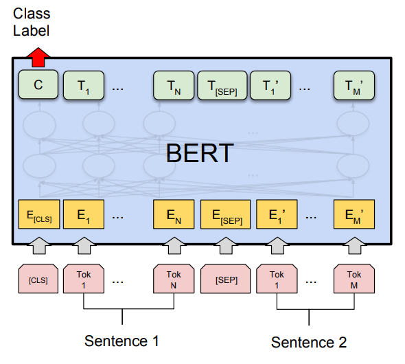
BERT (Bidirectional Encoder Representations from Transformers) is based on the Transformer architecture introduced by Vashwani et al. in 2017

MLM works by taking 15% of the text tokens that BERT sees and replacing them with a [MASK] token. The model’s objective is to predict that masked word with its embedding, using the context from the surrounding tokens, and then it is trained on the cross-entropy loss between the predictions and the actual truth.
BERT was also trained on the NSP (Next Sentence Prediction) objective. In training, the model is given a pair of input segments, and its task is to predict whether the second segment (segment B) follows the first one (segment A) in the original text or if they are randomly sampled and unrelated. The input is constructed by concatenating segment A, which is preceded by a special [CLS] token, and segment B, with a special [SEP] (separator) token in between. For example: “[CLS] Segment A [SEP] Segment B”. BERT then produces a pair of embeddings: one for the [CLS] token at the beginning of the input and one for the [SEP] token that separates the two segments. These embeddings are then used to compute a binary classification. The intended effect is that [CLS] contains information about the overall meaning of the first sentence, and [SEP] contains information about the second. This is the first example of sentence embeddings, which are the key to how a modern embeddings model works.
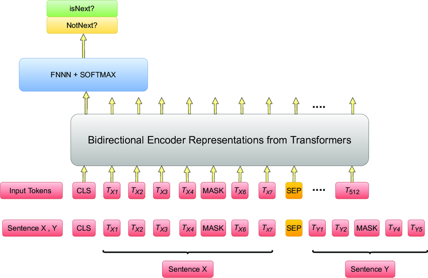
BERT turns token inputs into embeddings for each token in its context window, which is 512 tokens long. We can choose to construct a single text embedding from this any way we like. There are several popular strategies for this “token pooling” problem. Reading the above, one may be tempted to take the [CLS] token’s embedding. In practice, however, the [CLS] token embeddings proved to be slightly worse than just taking the average of all the individual token embeddings of the sentence
SBERT
The final part of the story is Sentence-BERT
This encourages the model to predict positive pairs (similar passages) as vectors with close to 1 similarity, and negative pairs close to 0. Similarity metrics include (Euclidean) distance, but most often used is cosine similarity. Negative pairs can either be “mined” with some heuristic such as bag-of-words, or simply sampled at random from other examples in the batch. Due to this, pretraining batch sizes for embedding BERTs are often huge, in the tens of thousands

The reason two models are used is that many tasks see improved performance if there is a distinction made between “questions” and “answers”. For example, searches and retrieval queries may not resemble the results they most need in meaning: “What is the the tallest building in Hong Kong” and “The International Commerce Centre” are not closely semantically related, but should be paired in search contexts. Because of this, we can train a “query” and “passage” model together as one giant network on a contrastive loss, and thus get a model that can take in both.
In practice, this improvement is rarely worth doubling the number of parameters, and so most papers simply re-use the same model for both queries and passages.
How Embeddings Models are Trained
Putting all this together, we have the current standard recipe for training a modern embeddings model, in up to three stages:
1. Pretraining
It is valuable to start with a language model that has already learned some inner representation of language. This makes the embeddings task significantly easier, since the model must only learn to condense this inner representation into a single high-dimensional dense vector space. While it is possible to use more modern LLMs such as GPT or LLaMA for embeddings
2. Training
Following Sentence-BERT, the model is trained contrastively. At this point, we choose a pooling strategy to convert BERT outputs into sentence embeddings. Many current papers choose to use average pooling
3. Fine-Tuning
It has also become common to fine-tune especially large embeddings models on higher-quality datasets, such as MS MARCO (Bing question-passage responses)
How Embeddings Models are Tested
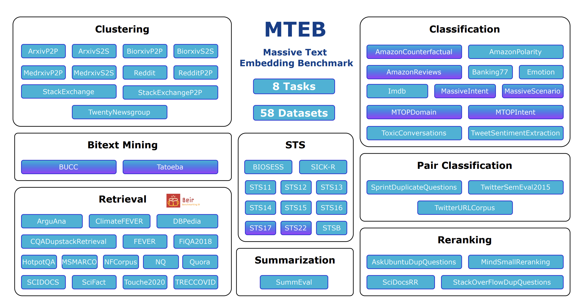
Similarly to how decoder LLMs have recently converged on being measured on the HuggingFace Open LLM Leaderboard, the currently ubiquitous benchmark for embeddings models is MTEB
-
Bitext Mining: Inputs are two sets of sentences from two different languages. For each sentence in the first set, the best match in the second set needs to be found. This metric is commonly ignored in places such as the MTEB Leaderboard and in papers, because few multilingual models have been created.
-
Classification: A train and test set are embedded with the provided model. The train set embeddings are used to train a logistic regression classifier, which is scored on the test set.
-
Clustering: Involves grouping a set of sentences or paragraphs into meaningful clusters. A k-means model is trained on embedded texts. The model’s performance is assessed using the v-measure, which is independent of the cluster labels.
-
Pair Classification: Requires assigning labels to pairs of text inputs, typically indicating if they are duplicates or paraphrases. Texts are embedded and distances calculated using various metrics (cosine similarity, dot product, Euclidean, Manhattan). Metrics like accuracy, average precision, F1, precision, and recall are used.
-
Reranking: Involves ranking query results against relevant and irrelevant reference texts. Texts are embedded using a model, with cosine similarity determining relevance. Rankings are scored using mean MRR@k and MAP, with MAP as the primary metric.
-
Retrieval: Each dataset includes a corpus and queries, with a goal to find relevant documents. Models embed queries and documents, computing similarity scores. Metrics like nDCG@k, MRR@k, MAP@k, precision@k, and recall@k are used, focusing on nDCG@10.
-
Semantic Textual Similarity (STS): Involves assessing the similarity of sentence pairs. Labels are continuous, with higher scores for more similar sentences. Models embed sentences and compute similarity using various metrics, benchmarked against ground truth using Pearson and Spearman correlations. Spearman correlation based on cosine similarity is the main metric.
-
Summarization: Evaluates machine-generated summaries against human-written ones. Models embed summaries, computing distances between machine and human summaries. The closest score, such as the highest cosine similarity, is used for evaluation. Metrics include Pearson and Spearman correlations with human assessments, focusing on Spearman correlation based on cosine similarity.
We can see that MTEB represents many downstream users’ desires as described earlier, but could be criticised for favoring cosine similarity as a distance metric for training. In either case, MTEB has demonstrated, and itself encouraged, some trends in research:
Scaling
The MTEB paper itself, as well as the GTR
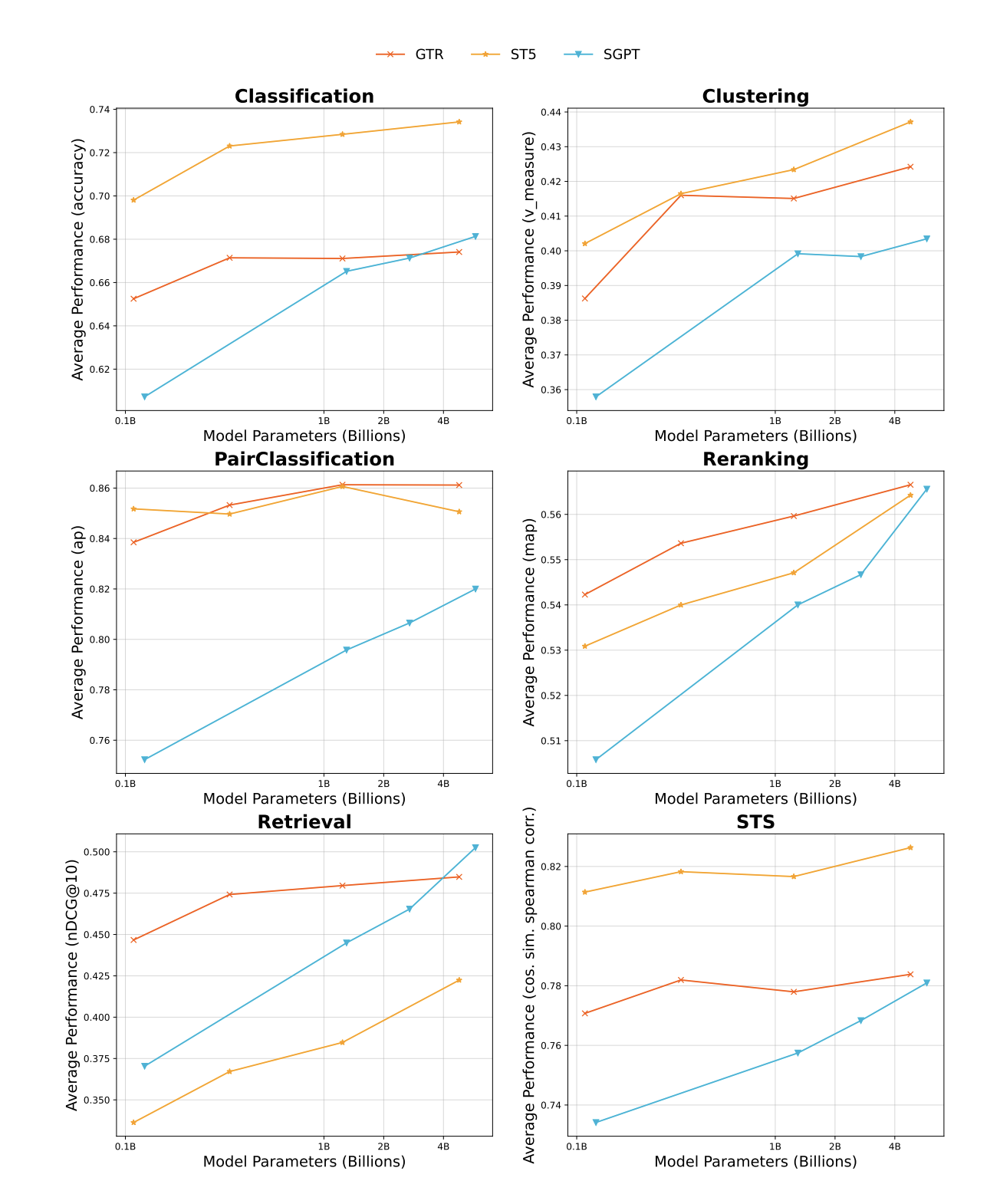
However, if we extrapolate to more recent research , we find that the state-of-the-art models have failed to get bigger over time, and the highest-performance models are still under 1B parameters. This shows that embeddings is not as easily reduced to scaling laws as LLMs are.
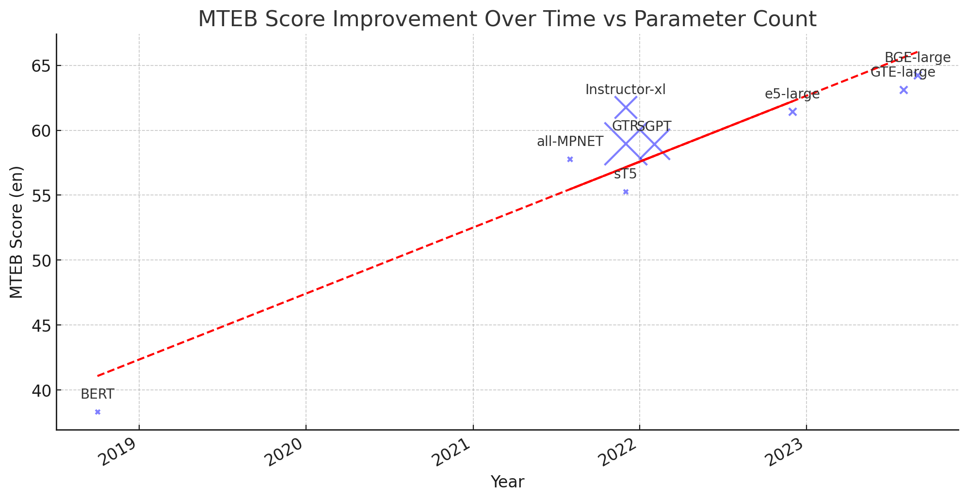
However, even these small models still train on hundreds of millions or billions of text pairs
Multilingualism
While MTEB is a multilingual benchmark, only a few tasks, namely STS, Classification and Bitext Mining, have multilingual versions. Combined with the abundance of English training data, this has led to every language except English, Chinese and Polish lacking a complete MTEB and thus lacking the benefits of state-of-the-art models.
As in other subfields of NLP, multilingual performance is often an afterthought, and left by the wayside in pursuit of higher performance on English benchmarks, or exclusively in the domain of labs that can afford extra runs
Method
With these problems as our motivation, we aim to find out if it is possible to add multilingualism to an existing model without having to pretrain from scratch. This may be a step towards bringing the benefits of increased embeddings performance to languages that don’t currently have a state-of-the-art model. Furthermore, if it is possible to add a new language to an existing model, this hints at the ideas that models do not necessary learn a representation based on a particular language, and that translation is easier than expected in the context of embeddings, modelable as a transformation of the representation space.
To do this, we will take an existing model that has both monolingual English and multilingual variants, and use contrastive training to add in new languages without sacrificing English performance, by using publicly available text translation pairs. We call this approach Cross-Lingual Fine-Tuning (CLFT). We will attempt to create a model that performs on-par with the multilingual model in multiple languages, and on-par with the original model in English, which we will measure by completing with our own data a multilingual version of MTEB in all tasks.
Model Choice
We choose e5-base-v2 and multilingual-e5-base
This choice does produce a caveat in the rest of our post - since the BERT tokenizer of e5-base has been trained only on English data, it will be unable to tokenize text that is not also a possible English string. In practice, this means that any Latin or near-Latin speaking languages, such as French, German and Turkish, can be used, but the model cannot be finetuned to read unknown characters like Japanese or Arabic script. Any non-Latin characters will likely become an [UNK] token, which carries no information for the model to embed. We are confident that this is not a fatal flaw, though, since just as it is possible to train LLMs with unused vocabulary, such as Persimmon-8B
Benchmarking
As described above, it is hard to use MTEB to test performance in non-English languages, due to the lack of available tasks. After investigating the source datasets, we know that this is because of a lack of data. In the interest of producing a universally fair test, especially for low-resource languages where quality data is not available, we opted to use synthetic data to create a multilingual MTEB test set, by using machine-translation to convert the English datasets into each language.
We used GPT 3.5 to process ~200K test examples in each of the following languages: French, German, Spanish, Swahili, and Turkish. We selected these languages because of their presence on the No Language Left Behind (NLLB) text-pair dataset
As mentioned before, MTEB already contains some multilingual components, in the textual similarity, bitext mining and classification tasks. The bitext mining task in particular requires a cross-lingual model, so we will use it only on the final all-language model. The remaining tasks are clustering, retrieval, classification, re-ranking, STS, and summarization. For each task, we selected one dataset that would generalise well across languages. Given more time and compute resources, it would be easy to expand the dataset to a full synthetic multilingual MTEB. From now on, we refer to this benchmark as MMTEB (Multilingual Massive Text Embeddings Benchmark).
Datasets and code for evaluation are available HERE.
| Task | Classification | Clustering | Retrieval |
|---|---|---|---|
| Dataset | MASSIVE | Reddit and TwentyNewsgroup | SciFact |
| Semantic Text Similarity | Summarization | Reranking | Pair Classification |
| STS-22 | SummEval | MIND | Twitter URL Corpus |
Training
In CLFT, we initialize two instances of our base model, one of which is frozen, and the other is trained. We will refer to these as $f_s$ and $f_\theta$ for the static and trained model. The static model will be used to anchor our trained model to the initial representation. For each lanuage $l$, our data $X_l$, is composed of pairs of data points $(x_e, x_l) \in X_l$, where $x_e$ is a sentence in english, and $x_l$ is that sentenced translated to language $l$.
We initially attempted to use the literature-standard InfoNCE
We give the model \(f_\theta\) the following goal: place \(x_l\) as close to \(x_e\) as possible, without changing where we place \(x_e\). This is crucial, because it forces the model to map the new language onto its existing representation. This is done with the following loss function
\[\mathcal{L}(x_e, x_f) = \mathcal{L}_{\text{eng}} + \beta \mathcal{L}_{\text{cross}}\]Where:
- \(\mathcal{L}_{\text{eng}} = 1 - f_\theta(x_e) \cdot f_s(x_e)\) represents the loss component for English text, with \(f_\theta\) as the dynamic model being trained and \(f_s\) as the static reference model.
- \(\mathcal{L}_{\text{cross}} = 1 - f_\theta(x_e) \cdot f_\theta(x_f)\) represents the cross-lingual consistency loss, comparing the dynamic model’s outputs for English and foreign text.
- \(x_e\) and \(x_f\) are inputs for English and foreign text, respectively.
- \(\beta\) is a coefficient to balance the influence of the cross-lingual consistency term.
We ran each of our mono-lingual models on 400,0000 text pairs from the NLLB
Results
We found interesting and surprising results across our chosen languages and tasks. The results in table format are available in the appendix.
We can visualize these results in two graphs: comparing our approach to the baseline English model, and to the current state-of-the-art multilingual model.
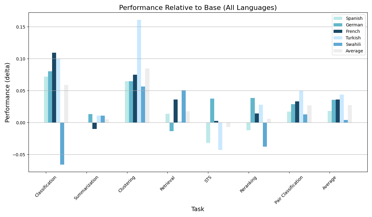
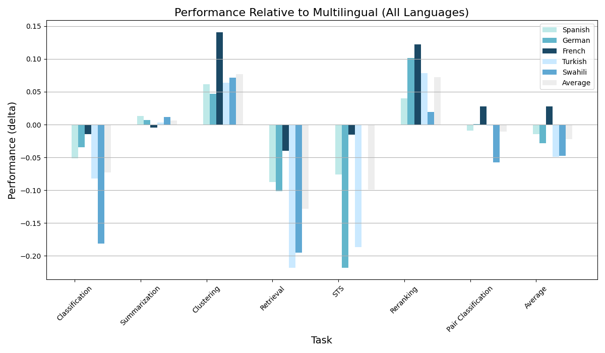
We can see that the CLFT approach did extremely well on tasks like classification, pair classification and clustering, even beating the multilingual model itself. This is to be expected in particularly well-suited tasks, since a perfect monolingual model will always outperform a multilingual model at a set number of parameters. However, the model did not improve as strongly in retrieval and semantic textual similarity tasks. Additionally, we can see the model struggle most significantly in Swahili, the most distant language to its original English in our training set. Overall, we observed an average 5.5% relative improvement on the base model, taking us 49.8% of the way to the performance of the multilingual model.
We have some conjectures about the reason for this split, which relate to the theory of representation learning. Since our loss is purely on positive pairs, there is weaker enforcement of a shape of the embeddings space. It is therefore likely that our approach is degenerating the shape of the embeddings space, leading to more clustering and noisier local structure. This means that tasks that rely on broad-strokes embeddings, such as clustering, classification and so on, will benefit from this approach, whereas tasks that rely on fine-grained relative positioning such as retreival, reranking and STS will suffer. CLFT could thus be viewed as a trade-off between speed and ease of training, and noisiness of embeddings.
We investigate this by performing a visual analysis of the embeddings after PCA dimension reduction. In the figure below, we see how different model represents the same text, after it has been translated. The texts were taken from the associated reddit clustering datasets for each language, and the labels in the diagrams are the name of the corresponding class of the datapoint. We see that the position of each embedding is roughly the same, which makes sense given our loss function.
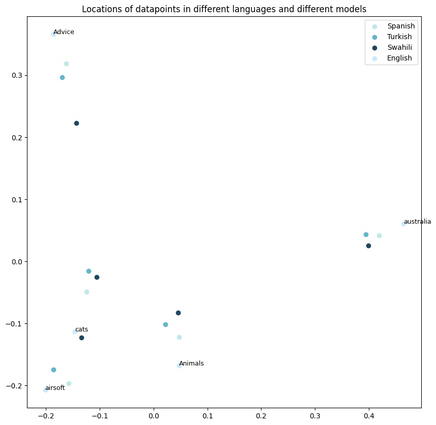
Additionally, the figure below demonstrates that we were mostly successful in our goal of keeping our trained models aligned with the underlying english model. We embedded the same, English text with each model and got an even tighter clustering. We see that the training on languages more similar to english, such as Spanish, did not alter the English represenations as significantly. Conversely, more distant languages, such as Swahili, led to further degradation of the embedding space.

Conclusions
Based on our results, we conclude that fine tuning for multilinguality is a cheap and viable alternative, especially when working with languages that do not have a large presence on the internet. While not an improvement over “true” multilingual models in general, CLFT can outperform multilingual models in scenarios where high-quality data is sparse, or in specific task categories (like clustering and reranking).
Additionally, we have made steps to introduce the first truly multilingual benchmark, for future embedding models to be evaluated against. All code and data for MMTEB assessment can be found here
Limitations and Next Steps
Our experiment has several limitations, and there is plenty of room for extension:
The fact that we used machine-translated English text for our benchmark poses potential issues. It’s likely that the distribution of data that our translation model produces is not equivalent to that produced in the real world, meaning that our benchmark isn’t as accurate as the English one is. This is hard to ameliorate, especially for languages lacking many large datasets. However, barring vast troves of previously undiscovered internet data being discovered, translations can serve as a useful stopgap, and an equalizer for these less available languages. Completing the MMTEB benchmark would be a valuable contribution to the field, and a path to more languages being represented in state-of-the-art models.
In this paper, we only evaluated monolingual models, and did not study how the approach scales to multiple languages at once. Due to time and compute constriants, we were unable to try and train a “true” multilingual model, beyond just english and one other language. We believe that with further training, it may be possible to repeat the process above for multiple languages.
As mentioned in our results, CLFT can lead to noisy embeddings, which may decrease performance on particular tasks. A better distillation loss, or traditional contrastive loss with a much larger batch size, may help to regularize the data and resolve this issue.
As previously mentioned, we could not explore non-latin characters, vastly reducing our set of potential languages. We believe that with the correct tokenizer and base model, this should be possible. Additionally, it’s becoming possible to imagine a future of Transformers without tokenization, which would greatly help approaches like ours.
Despite our models maintaining near perfect alignment with the base model on the english text pairs during training, we observed performance on the English MTEB decrease substantially. This suggests that the text pairs on NLLB do not fully capture the distribution of data seen during testing,which is something that could be improved upon with better translation datasets.
Appendix
Here is a full table of our results:
| Classification | Summarization | Clustering | Retrieval | STS | Reranking | Pair Classification | Average | |
|---|---|---|---|---|---|---|---|---|
| Spanish (e5-base) | 0.511 | 0.314 | 0.333 | 0.554 | 0.585 | 0.296 | 0.828 | 0.489 |
| Spanish (e5-multi) | 0.635 | 0.301 | 0.336 | 0.655 | 0.629 | 0.243 | 0.848 | 0.521 |
| Spanish (ours) | 0.583 | 0.314 | 0.398 | 0.568 | 0.553 | 0.284 | 0.847 | 0.507 |
| German (e5-base) | 0.522 | 0.307 | 0.328 | 0.560 | 0.236 | 0.293 | 0.812 | 0.437 |
| German (e5-multi) | 0.637 | 0.313 | 0.346 | 0.648 | 0.491 | 0.230 | 0.840 | 0.501 |
| German (ours) | 0.602 | 0.320 | 0.393 | 0.546 | 0.273 | 0.332 | 0.841 | 0.472 |
| French (e5-base) | 0.512 | 0.312 | 0.329 | 0.568 | 0.747 | 0.330 | 0.825 | 0.518 |
| French (e5-multi) | 0.637 | 0.306 | 0.263 | 0.644 | 0.764 | 0.222 | 0.845 | 0.526 |
| French (ours) | 0.622 | 0.302 | 0.404 | 0.604 | 0.749 | 0.344 | 0.849 | 0.554 |
| Turkish (e5-base) | 0.458 | 0.296 | 0.221 | 0.411 | 0.456 | 0.308 | 0.776 | 0.418 |
| Turkish (e5-multi) | 0.639 | 0.304 | 0.318 | 0.631 | 0.601 | 0.258 | 0.827 | 0.511 |
| Turkish (ours) | 0.557 | 0.307 | 0.382 | 0.413 | 0.414 | 0.336 | 0.826 | 0.462 |
| Swahili (e5-base) | 0.413 | 0.304 | 0.181 | 0.281 | 0.000 | 0.313 | 0.751 | 0.321 |
| Swahili (e5-multi) | 0.528 | 0.303 | 0.166 | 0.527 | 0.000 | 0.257 | 0.822 | 0.372 |
| Swahili (ours) | 0.347 | 0.315 | 0.238 | 0.332 | 0.000 | 0.275 | 0.764 | 0.325 |
| Average (e5-base) | 0.483 | 0.307 | 0.279 | 0.475 | 0.405 | 0.308 | 0.799 | 0.436 |
| Average (e5-multi) | 0.615 | 0.306 | 0.286 | 0.621 | 0.497 | 0.242 | 0.836 | 0.486 |
| Average (ours) | 0.542 | 0.312 | 0.363 | 0.493 | 0.398 | 0.314 | 0.825 | 0.464 |