Learning Interpretable Features with Sparse Auto-Encoders
Introduction
The field of Machine Learning is becoming increasingly promising as humanity endeavors to create intelligent systems, with models outperforming humans on many tasks. As models become increasingly capable, its important that humans are able to interpret a model’s internal decision making process to mitigate the risk of negative outcomes. While significant progress has been made on interpreting important parts of models like attention heads
Superposition Hypothesis
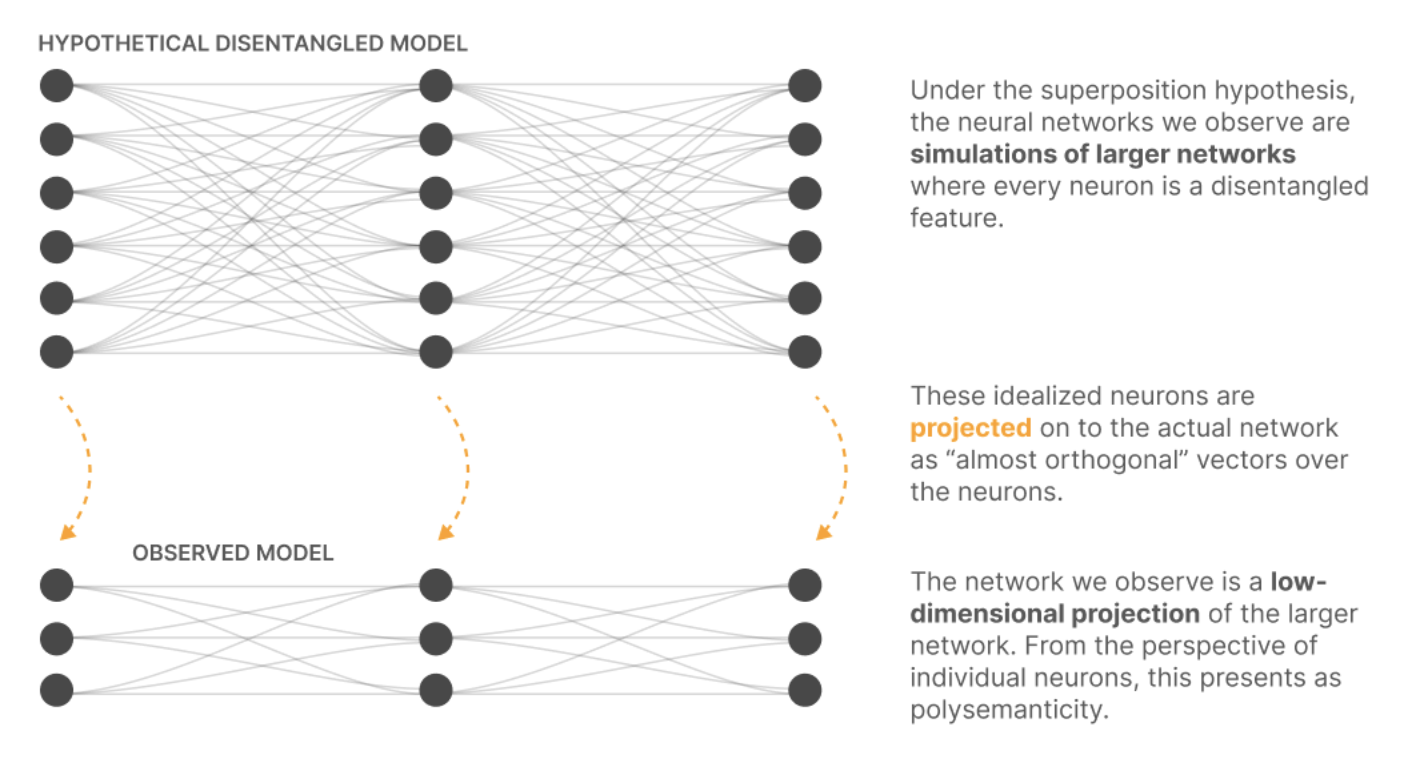
One hypothesis for why it can be challenging to interpret individual neurons is because they are simultaneously representing multiple concepts. One may wonder why a network would have its neurons learn to represent multiple concepts. At a first glance, this approach to encoding information feels unintuitive and messy. The key idea comes from the Johnson–Lindenstrauss lemma: In $n$ dimensions, you can have at most $n$ pairwise orthogonal vectors, but the number of pairwise “almost orthogonal” vectors (i.e. cosine similarity at most $\epsilon$) you can have is exponential in $n$. This enables a layer to encode for many more concepts than it has neurons. So long as each neuron is only activated by a sparse combination of concepts, we can reconstruct these concepts from a given activation with minimal interference between the concepts, since they are “almost orthogonal”. This hypothesis is known as superposition
Sparse Auto-Encoders
Since deep neural networks are strongly biased towards making neurons polysemantic during training, humans might try to understand the model’s decision making process by “unwrapping” the network into the sparse features that the neurons in some particular layer are simulating. To do this, a concept called a Sparse Auto-Encoder (SAE) is used. An SAE is similar to a normal autoencoder, with two main differences: (1) the encoding layer is larger than the neuron layer, often by a factor of 4x. (2) the loss function penalizes not only for the MSE loss, but also for the sparsity of the encoder matrix, frequently represented as L1 loss. A sparse autoencoder lets us learn a sparse representation for a vector, but in a higher dimensional space. SAEs were first proposed in a blogpost by Lee Sharkey in December 2022, and in September 2023 more research was published on SAEs, both by a group of independent researchers

Research Question
This inspired a new idea: what if we could take a neural network, unwrap each layer into a larger, sparse, interpretable set of features, and then learn a sparse weight matrix connecting all pairs of two consecutive feature layers? This would mean that we could take a neural network, and transform it into a new neural network simulating the old neural network, with the nice property that the computations are sparse and hopefully interpretable.
The main question we wish to explore is: Can we unwrap a deep neural network into a larger sparse network and learn sparse weights between consecutive feature layers without losing performance?
Initial Mathematics
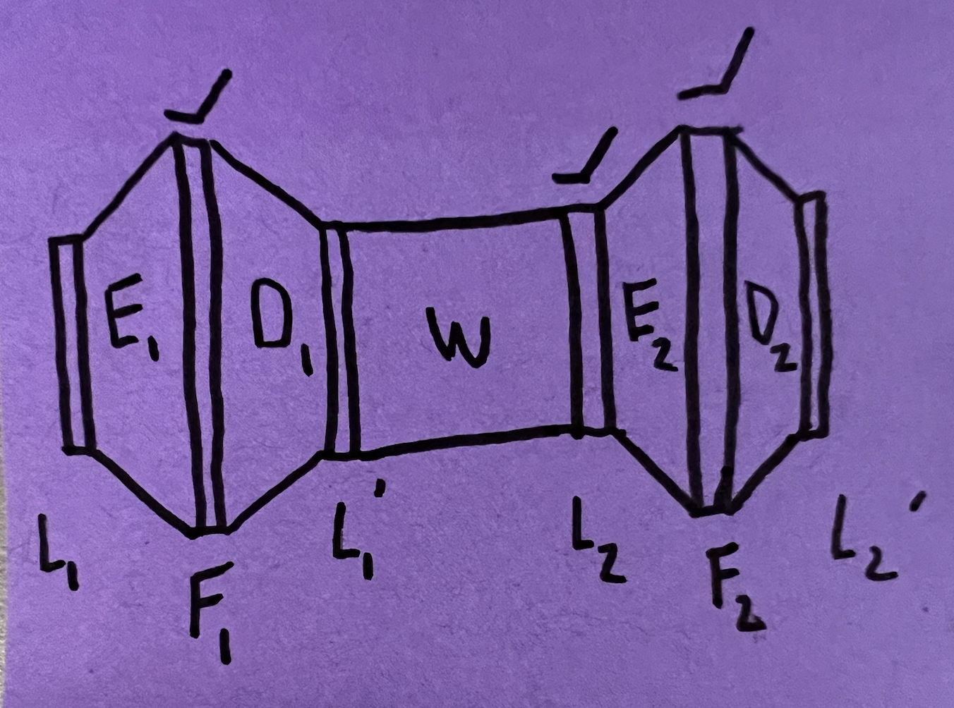
Let’s begin by looking at $L_1$ and $L_2$, two consecutive layers in a deep neural network with ReLU activations. Let $W$ and $b$ be the matrix and bias respectively that connects these two layers. Then we have
\[L_2 = \text{ReLU}(W L_1 + b)\]We create autoencoders such that
\[L_1 = D_1 \text{ReLU}(E_1 L_1 + e_1) \equiv D_1 F_1\] \[L_2 = D_2 \text{ReLU}(E_2 L_2 + e_2) \equiv D_2 F_2\]where $D_i$ is the decoder for layer $i$, $E_i$ and $e_i$ are the weights of the encoder and encoder bias, and $F_i$ is the feature vector.
Thus we have
\[\begin{align} F_2 &= \text{ReLU}(E_2 L_2 + e_2) \\ &= \text{ReLU}(E_2 \text{ReLU}(W L_1 + b) + e_2) \\ &= \text{ReLU}(E_2 \text{ReLU}(W D_1 F_1 + b) + e_2). \end{align}\]In general, an approximation of the form
\[F_2 = \text{ReLU}(W_2 F_1 + b_2)\]would be pretty terrible since we cannot easily approximate a double ReLU function with a single ReLU function. However, because of the way $F_1$ and $F_2$ are created from $L_1$ and $L_2$, the relationships are actually very sparse in nature, so we will try to learn the approximation above. Perhaps there is a clever initialization that will allow us to learn this more easily.
If we just ignored the inside ReLU in the definition of $F_2$, then we’d have
\[F_2 = \text{ReLU}(E_2 W D_1 F_1 + E_2 b + e_2)\]which suggests the following could be a good initialization for our learned weight $W_2$ and bias $b_2$.
\[W_2 = E_2 W D_1\] \[b_2 = E_2 b + e_2\]While this initialization seemed reasonable at the start of the project, it turned out that during training this results in a local minimum, and you can actually get much lower loss if you randomly initialize $W_2$ and $b_2$.
Codebase
To answer this main question, the first step was to build out a codebase that had all the implementations necessary to run experiements to explore this question. The codebase was developed from scratch to ensure I understood how each part of the code worked.
Model
The first part of the code trains a four layer neural network to classify MNIST images. After training we got a validation loss of 0.09 and a validation accuracy: 0.98, indicating the model does well. For clarity, all losses described in this section will refer to loss on the validation set.
SAEs
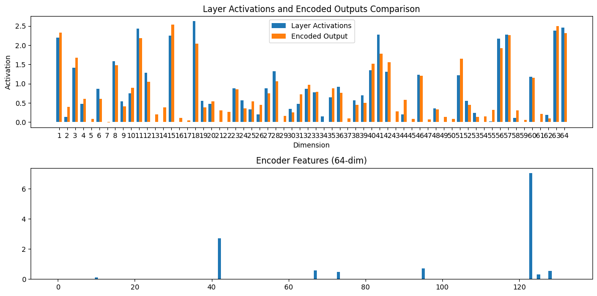
Next, two autoencoder architectures are implemented, one that learns both an encoder and decoder, and one that learns only an encoder as its decoder is tied as the transpose of the encoder. Empirically, the tied autoencoder seemed to perform better and achieved an L1 (sparsity) loss of 0.04928, and an L2 (MSE) loss of 0.03970. Seeing these numbers close in magnitude is good, indicating that the model is neither penalizing too much nor too little for L1 sparsity loss.
Feature Connectors
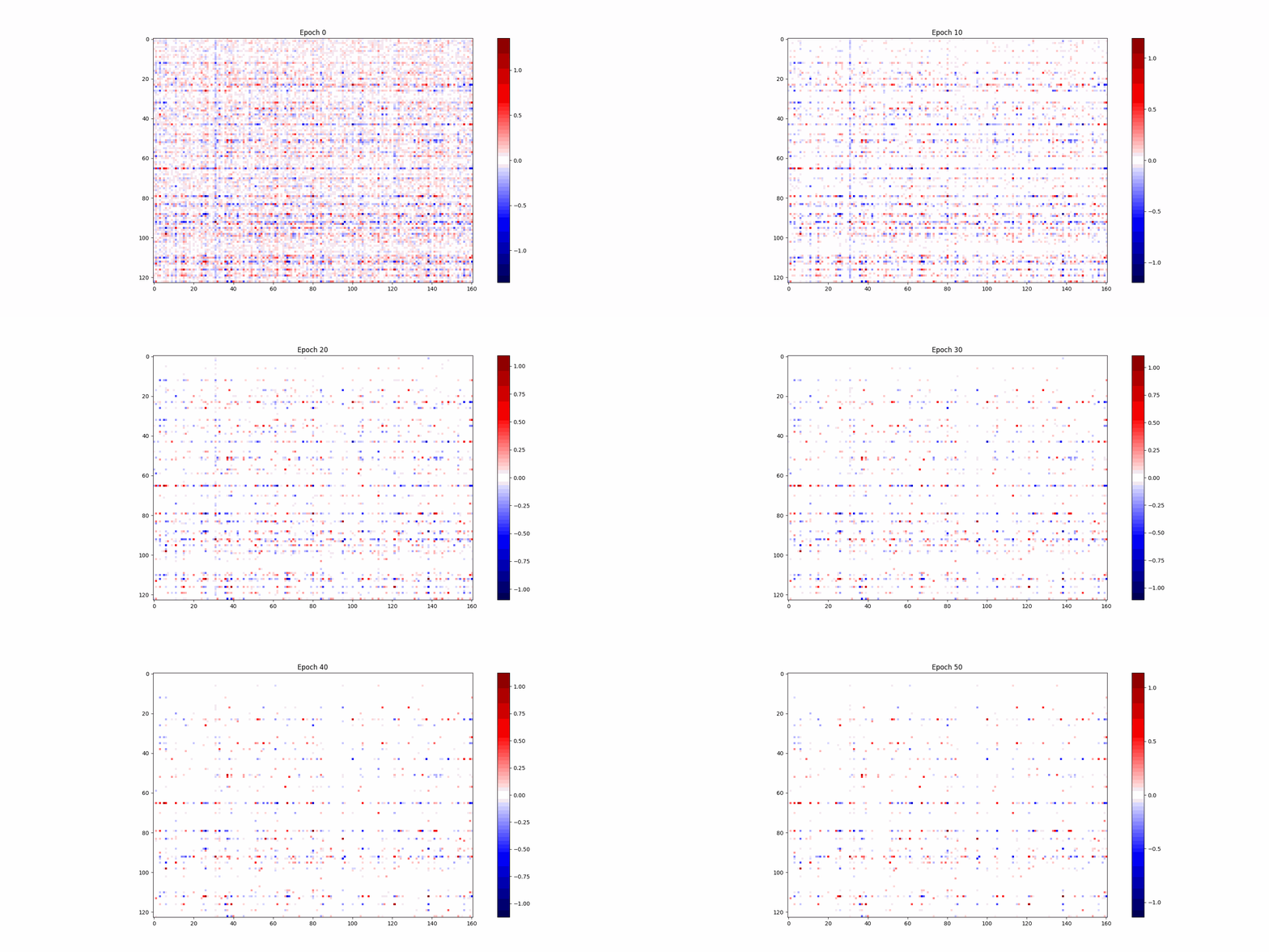
Then, a feature connector was implemented, which learns the matrices $W_2$ and $b_2$ descibed above mapping one layer to another layer. The inputs are the set of all feature $i$ activations and the outputs are the set of all feature $i+1$ activations, allowing us to gradient descent over loss (which consists of L1 sparsity and L2 MSE) to optimize $W_2$ and $b_2$. The L1 (sparsity) loss was 0.02114 and the L2 (MSE) loss: 0.03209, indicating that there is a good tradeoff between L1 and L2 penalty.
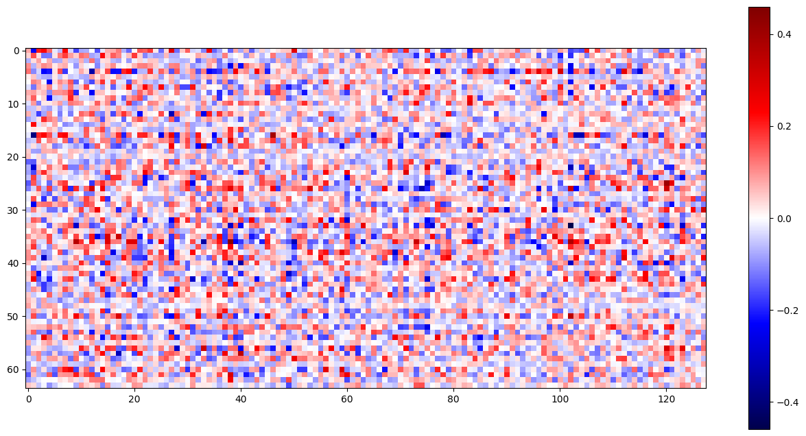
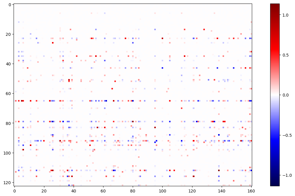
Below is what the feature connector matrix looks like after each epoch of training.
Simulating the Feature Network
Finally, we replace neuron connections with feature connections. This means that when we pass an input through the network, we immediately encode it as a feature and propogate it through the feature connector weights, skipping the neuron layer weights. In this network, removing two neuron to neuron layers and substituting them with feature to feature layers results in a decrease from 97.8% accuracy to 94% accuracy, which is pretty good considering we made our network much sparser.
Next, I tried to visualize the features using a variety of methods (both inspired by a class lecture and a Distill blogpost
Language Models
I shared these results with Logan Riggs, one of the independent researchers
Below we show some examples of sparse linear feature connections. For the curious reader, additional examples can be found here.
OR Example
In Layer 1, we have:
\[OF_{30} = 0.26IF_{2797} + 0.23IF_{259} + 0.10IF_{946}\]where OF is output feature (in MLP_out), and IF is input feature (in Residual Stream before the MLP)
Below is input feature 2797, activating strongly on the token “former”

Below is input feature 259, activating strongly on the token “old”

Below is input feature 946, activating on the token “young”

In the output feature, we see the tokens former, old, and young all activate, with young activating about half as strongly as “former” and “old” as we would expect from the weight coefficients.
\(OF_{30} = 0.26IF_{former} + 0.23IF_{old} + 0.10IF_{young}\)

We can view this computation as a weighted logical OR. Output Feature 30 activates on former OR old OR young.
Negative Weight Example
In Layer 1, we have:
\[OF_{505} = 0.68IF_{3021} -0.21IF_{729}\]where OF is output feature, and IF is input feature.
Below is input feature 3021, activating strongly on tokens like “said” which in almost all cases appear not after a quote.

Below is input feature 729, activating strongly on tokens like “said” when they appear shortly after a quote.

Below we see the output feature activates on tokens like “said” that have no prior quote tokens. We’ve “subtracted out” with a large negative weight, so to speak, the examples where “said” appears after a quote, and now the feature only activates when “said” appears without any prior quotes.
\[OF_{505} = 0.68IF_{(\text{"said" in many contexts})} -0.21IF_{(\text{"said" after quotes})}\]
We can view this computation as a weighted logical AND. Output Feature 505 activates on A AND ~B. In the case where A is a superset of B, this is the complement of B e.g. I have the set of all fruits and all yellow fruits, so now I can find all non-yellow fruits.
Conclusion
Our exploration into interpreting neural networks using Sparse Auto-Encoders has shown promising results. The ability to unwrap the layers of a neural network into a more interpretable, sparse representation without a significant loss in performance supports the superposition hypothesis. Even if the features were only interpretable on some architectures/datasets, I am optimistic that Sparse Auto-Encoders will not only make deep neural networks more interpretable, but they will also allow for quicker parallelized inference since each output feature will depend on a small fraction of the total possible input features.
I’d like to thank everyone who has contributed to my deep learning education this semester. I have learned a tremendous amount and really enjoyed working on this project.