Exploring the latent space of text-to-image diffusion models

In this blog post we explore how we can navigate through the latent space of stable diffusion and using interpolation techniques.

Introduction

Diffusion models are a class of deep generative models that have shown promising results in many different tasks, including photorealistic image generation and protein design . Diffusion models work by gradually destroying structure of an object with $T$ steps of a fixed noising process, and then learning to reverse this process to recover the original object. This allows the model to learn the underlying structure of the data, and to generate new objects that are both realistic and diverse. The forward process $q( x_t | x_{t-1} )$ defines how noise is added to an original image $x_0$, and the reverse process $q( x_{t-1} | x_{t} )$ that we want to learn, can recover a less noisy version of an image.

Stable Diffusion (SD) is an open-source latent text-to-image diffusion model which is able to realize images with fine grained details, when prompted with a textual input describing the desired characteristics of the output image. SD is reasonably fast compared to other diffusion models, since it performs the diffusion steps in a low dimensional latent space. The strategy consists of using an image encoder $\mathcal{E}: \mathcal{X} \rightarrow \mathcal{Z}^0$ which maps an image $x_0 \in \mathcal{X}$ to a lower dimensional image latent code $z_0 \in \mathcal{Z}^0$, and a latent decoder $\mathcal{D}: \mathcal{Z}^0 \rightarrow \mathcal{X}$ which recovers an image $\mathcal{D}(z_0)$ from the image latent code $z_0$. Using these two models it is possible to learn to denoise $z_T$, instead of $x_T$, which is also normally distributed, saving a lot in computing since the latent codes dimensionality are usually chosen to be much smaller than the original images dimensionality. During inference time, for a given input textual prompt $y$, we encode the prompt into a vector $s = \tau_\phi(y)$ using CLIP , sample $z_T \sim \mathcal{N}(0, I)$, and provide these two tensors to the diffusion model $f_\theta: \mathcal{Z}^T \times \mathcal{S} \rightarrow \mathcal{Z}^0$, which generates $z_0 = f_\theta(z_T, s)$. We can then map this vector into an image using the decoder: $x_0 = \mathcal{D}(z_0)$ which hopefully is in the data distribution.

Background and related work

In order to be able to learn the complex interaction between textual descriptions and images coming from a very large multimodal dataset, SD has to organize its image latent space $\mathcal{Z}^T$ coherently. If the learned representations are smooth for instance, we could expect that $\mathcal{D}(f_\theta(z_T, s))$ and $\mathcal{D}(f_\theta(z_T + \epsilon, s))$, where $\epsilon$ is a tensor of same dimensionality as $z_T$ with values very close to 0, will be very similar images. A common technique to explore and interpret the latent space of generative models for images is to perform latent interpolation between two initial latent codes, and generate the $N$ images corresponding to each of the interpolated tensors. If we sample $z_\text{start}, z_\text{end} \sim \mathcal{N}(0, I)$, fix a textual prompt such that $s = \tau_\phi({y})$ and use SD to generate images conditioned on the textual information we could explore different techniques for generating interpolated vectors. A very common approach is linear interpolation, where for $\gamma \in [0, 1]$ we can compute:

\[z_\text{linear}^{(\gamma)} = (1-\gamma)z_\text{start} + \gamma z_\text{end}\]

Mimicking these exact steps for three different pairs sampled latent codes for $(z_\text{start}, z_\text{end})$, and for each of them fixing a text prompt we get:

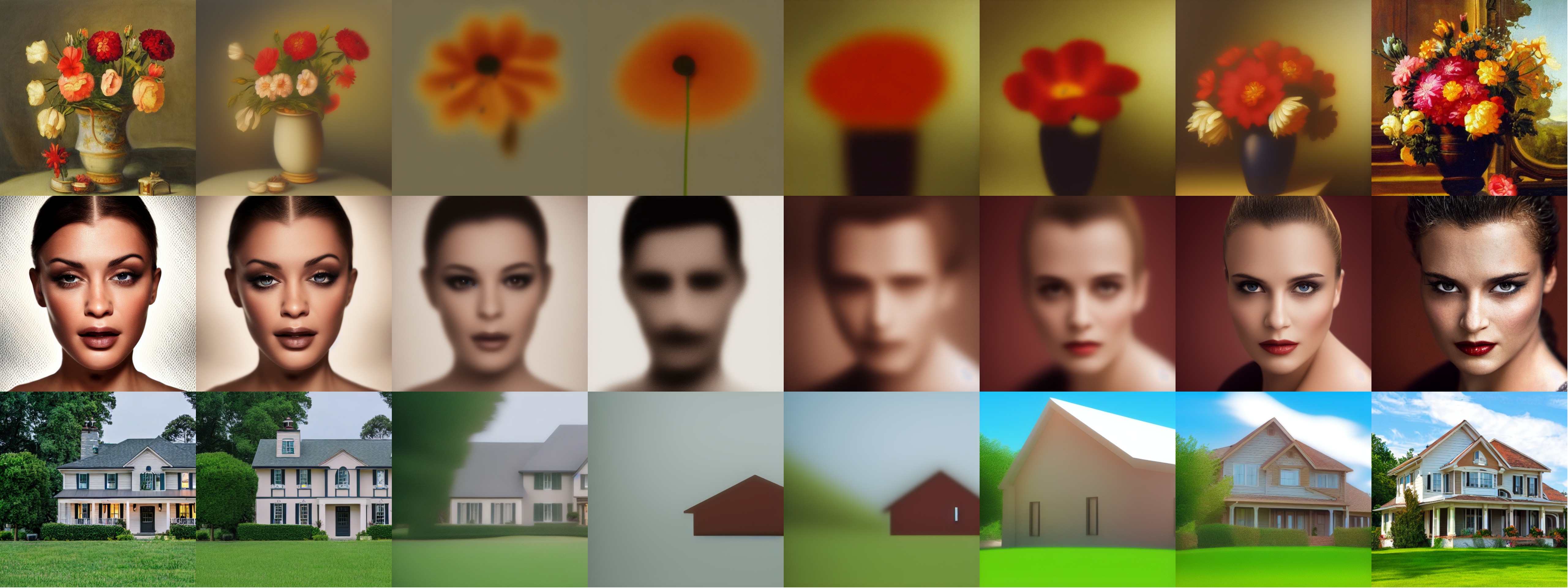
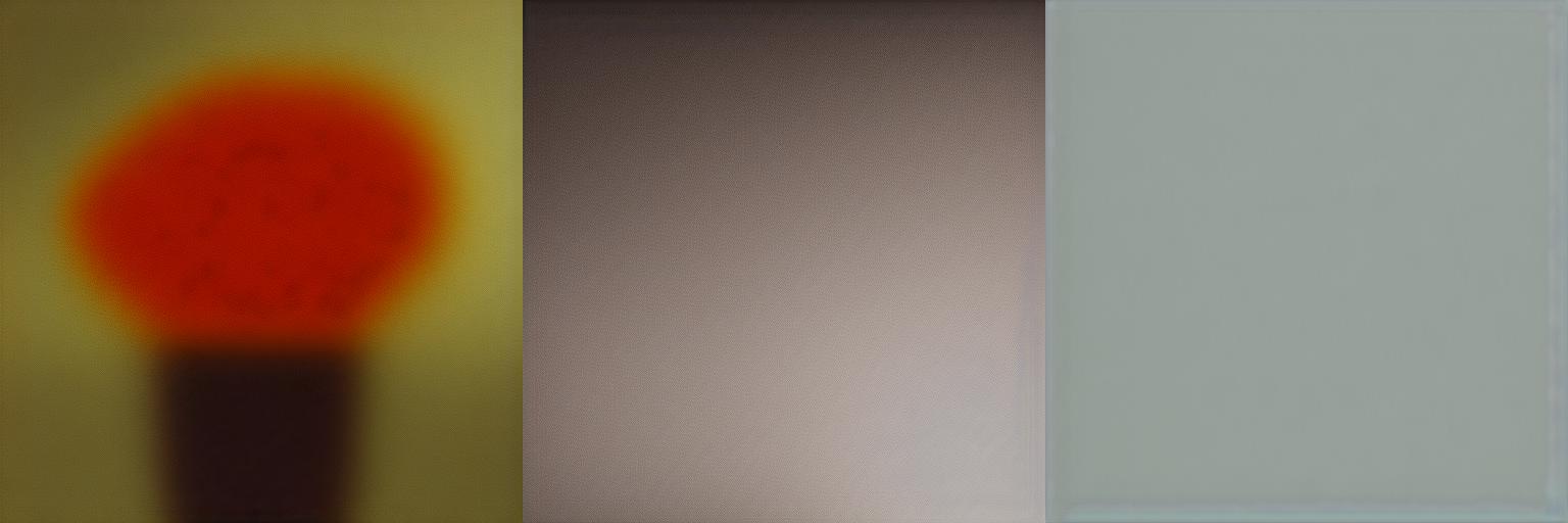
As we can see from the image, when we move away from both $z_\text{start}$ and $z_\text{end}$ we get blurred images after decoding the interpolated image latent codes, which have only high level features of what the image should depict, but no fine grained details, for $\gamma = 0.5$ for instance, we get:

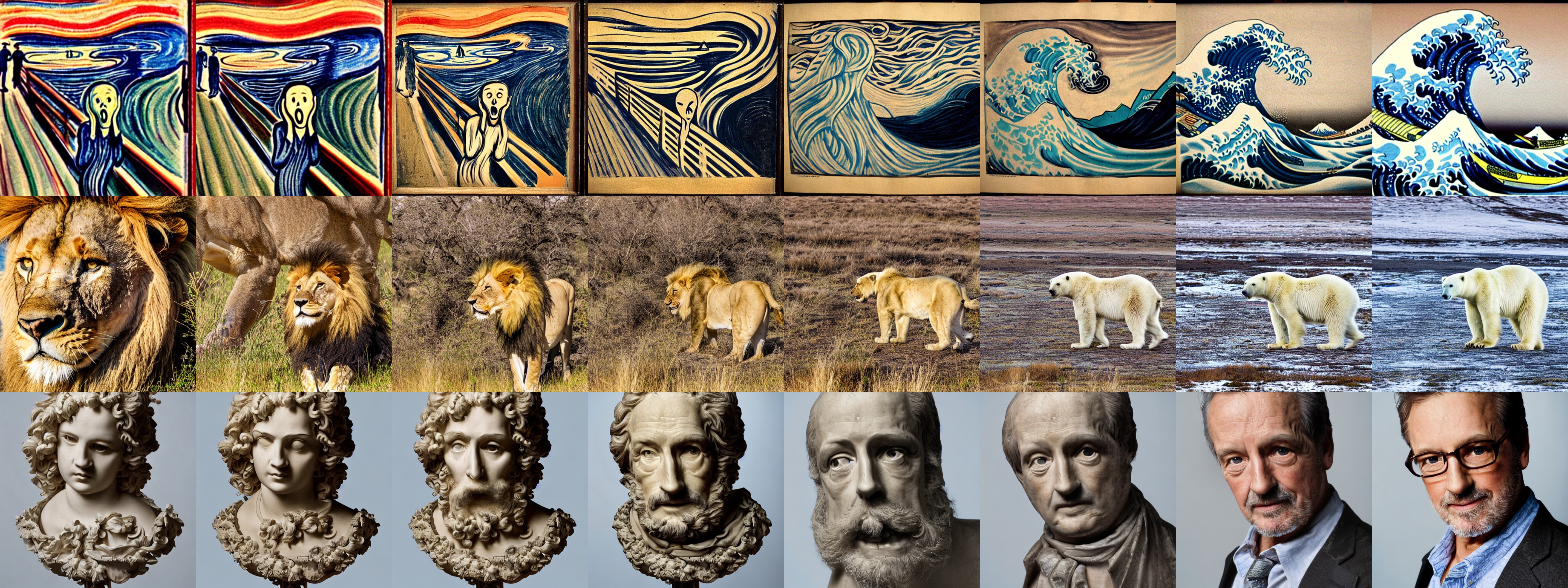
In contrast, if we perform interpolation in the text space by sampling $z_T \sim \mathcal{N}(0, I)$, which is kept fixed afterwards, and interpolating between two text latent codes $s_\text{start} = \tau_\phi(y_\text{start})$ and $s_\text{end} = \tau_\phi(y_\text{end})$, we get something more coherent:

Latent interpolation is a very common technique in Machine Learning, particularly in generative models, used interpolation in the latent space of a Variational Autoencoder (VAE) to generated molecules between two initial ones by encoding them in the VAE latent space, interpolating between them and using the decoder to obtain the molecules from the latents, showed how interpolation can be used to perform semantic transformations on images, by changing features of a CNN. More broadly interpolation has also been studied in a probabilistic point of view , evaluating how different techniques might generate out of distribution samples, which we explore later in this blog post.

In this project we explore geometric properties of the image latent space of Stable Diffusion, gaining insights of how the model organizes information and providing strategies to navigate this very complex latent space. One of our focuses here is to investigate how to better interpolate the latents such that the sequence of decoded images is coherence and smooth. Depending on the context, the insights here could transferred to other domains as well if the sampling process is similar to the one used in SD. The experiments are performed using python and heavily relying on the PyTorch , Transformers and Diffusers libraries.

Method

In this section we compare several interpolation techniques. For reproducibility reasons we ran the experiments with the same prompt and sample latent vectors across different. We use Stable Diffusion version 1.4 from CompVis with the large CLIP vision transformer, the DPMSolverMultistepScheduler , 30 inference steps and a guidance scale of 7.5 . We use the prompt “An high resolution photo of a cat” and seed = 1 to generate both $z_\text{start}$ and $z_\text{end}$. The corresponding generated pictures are shown below:

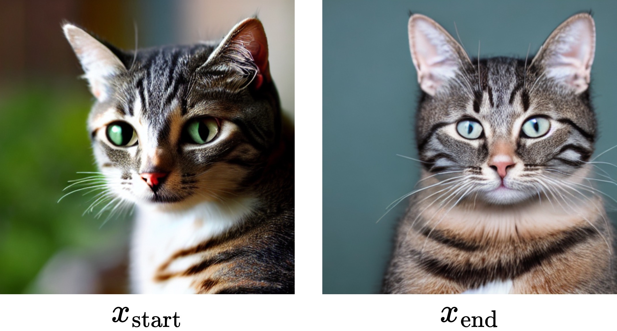
Linear Interpolation

Although linear interpolation is still a very commonly used interpolation technique, it is known that is generates points which are not from the same distribution than the original data points depending on the original distribution of the points being interpolated. Particularly, for $z_{\text{start}}, z_{\text{end}} \sim \mathcal{N}(0, I)$ and $\gamma \in [0,1]$, we have:

\[z_\text{linear}^{(\gamma)} = (1-\gamma)z_\text{start} + \gamma z_\text{end}\]

Hence:

\[\begin{eqnarray} \mathbb{E}\left[z_\text{linear}^{(\gamma)}\right] &=& \mathbb{E}\left[(1-\gamma)z_\text{start} + \gamma z_\text{end}\right] \nonumber \\ &=& \mathbb{E}[(1-\gamma)z_\text{start}] + \mathbb{E}[\gamma z_\text{end}] \nonumber \\ &=& (1-\gamma)\mathbb{E}[z_\text{start}] + \gamma \mathbb{E}[z_\text{end}] \nonumber \\ &=& 0 \nonumber \end{eqnarray}\]

Therefore, the mean stays unchanged, but the variance is smaller than 1 for $\gamma \in (0,1)$:

\[\begin{eqnarray} \text{Var}[z_\text{linear}^{(\gamma)}] &=& \text{Var}[(1-\gamma)z_\text{start} + \gamma z_\text{end}] \nonumber \\ &=& \text{Var}[\gamma z_\text{start}] + \text{Var}[(1-\gamma)z_\text{end}] \nonumber \\ &=& \gamma^2\text{Var}[z_\text{start}] + (1-\gamma)^2\text{Var}[z_\text{end}] \nonumber \\ &=& \gamma(2\gamma - 2)I + I \nonumber \\ &=& (\gamma(2\gamma - 2) + 1)I \nonumber \end{eqnarray}\]

Given that the sum of two independent Gaussian distributed random variables results in a Gaussian distributed random variable, $z_\text{linear}^{(\gamma)} \sim \mathcal{N}(0, (\gamma(2\gamma - 2) + 1)I)$. This shows how the distribution of the interpolated latent codes change. To further understand the effect of this shift, we can use the interactive figure below. Where for $\text{std} \in [0.5, 1.5]$ we generate an image using the embedding $\text{std} \, z_\text{start}$:

Normalized linear interpolation

As shown before, linear interpolation is not a good technique for interpolation random variables which are normally distributed, given the change in the distribution of the interpolated latent vectors. To correct this distribution shift, we can perform a simply normalization of the random variable. We will refer this this as normalized linear interpolation. For $\gamma \in [0,1]$ we define $z_\text{normalized}^{(\gamma)}$ as:

\[z_\text{normalized}^{(\gamma)} = \dfrac{z_\text{linear}^{(\gamma)}}{\sqrt{(\gamma(2\gamma - 2) + 1)}} \implies z_\text{normalized}^{(\gamma)} \sim \mathcal{N}(0, I)\]

Now, as we move further way from the endpoints $z_\text{start}$ and $z_\text{end}$, we still get coherent output images:

SLERP

Spherical Linear Interpolation (Slerp) , is a technique used in computer graphics and animation to smoothly transition between two orientations, especially rotations. If we let $\phi = \text{angle}(z_\text{start}, z_\text{start})$, then for $\gamma \in [0,1]$, the interpolated latent is defined by:

\[\text{slerp}(z_\text{start}, z_\text{end}; t) = \dfrac{\sin((1-\gamma)\phi)}{\sin(\phi)}z_\text{start} + \dfrac{\sin(\gamma\phi)}{\sin(\phi)}z_\text{end}\]

where $\phi$ is the angle between $z_\text{start}$ and $z_\text{end}$. The intuition is that Slerp interpolates two vectors along the shortest arc. We use an implementation of Slerp based on Andrej Karpathy . As we can see from the images below, slerp generates very good quality interpolated vectors.

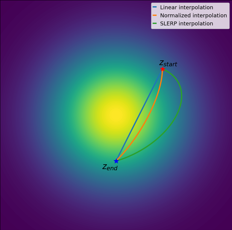
If we compare the obtained results with normalized linear interpolation we see that the generated images are very similar, but as opposed to normalized linear interpolation, we cannot easily theoretically analyze the distribution of generated latents. To have some intuition behind how these different techniques interpolate between two vectors and can sample and fix two vectors sampled from a 2-dimensional normal distribution. We can visualize how these trajectories compare with each other:

Translation

To further investigate some properties of the latent space we also perform the following experiment. Let $z_\text{concat} \in \mathbb{R}^{4 \times 64 \times 128}$ be the concatenation of $z_\text{start}$ and $z_\text{end}$ over the third dimension. We will denote by $z_\text{concat}[i, j, k] \in \mathbb{R}$ as a specific element of the latent code and $:$ as the operator that selects all the elements of that dimension and $m:n$ the operator that selects from elements $m$ to element $n$ of a specific dimension. We can create a sliding window over the concatenated latent and generated the corresponding images. We define the translation operator $\mathcal{T}$ such that $\mathcal{T}(z_\text{concat}; t) = z_\text{concat}[:, :, t:64+t]$, which is defined for $t = {0, \cdots, 64}$. The sequence of generated images can be visualized below using our interactive tool:

Surprisingly, we note that applying $\mathcal{T}$ to our concatenated latent code is materialized into a translation in image space as well. But not only the object translates, we also see changes in the images style, which is justified by changing some of the latent dimensions.

We can correct this behavior by mixing the two latent codes only in a single slice of the latent code. Let $\mathcal{C}(z_\text{start}, z_\text{end}; t)$ represent the concatenation of $z_\text{start}[:, :, 64:64+t]$ and $z_\text{end}[:, :, t:64]$ along the third dimension. With this transformation we obtain the following:

Hence, translation is also a valid interpolation technique and could be further expanded to generate an arbitrary size of latent vectors.

Analysis

In order to evaluate the quality of the generated interpolations we use CLIP, a powerful technique for jointly learning representations of images and text. It relies on contrastive learning, by training a model to distinguish between similar and dissimilar pairs of images in a embedding space using a text and an image encoder. If a (text, image) pair is such that the textual description matches the image, the similarity between the CLIP embeddings of this pair should be high:

\[\text{CLIPScore(text,image)} = \max \left(100 \times \dfrac{z_{\text{text}} \cdot z_{\text{image}}}{ \lVert z_{\text{text}} \rVert \lVert z_{\text{image}} \rVert}, 0 \right)\]

For each interpolation strategy $f \in \{\text{linear}, \text{normalized}, \text{slerp}\}$ presented, we fix the prompt $\text{text} = $ “A high resolution image of a cat” and generate $n = 300$ interpolated latents $f(z_\text{start}, z_\text{end}, \gamma) = z_f^{(\gamma)}$ with $\gamma = \{0, \frac{1}{n-1}, \frac{1}{n-2}, \cdots, 1\}$. We then generate the images $x_f^{(\gamma)}$ from the interpolated latents, finally we use the CLIP encoder $\mathcal{E}_\text{CLIP}$ on the generated images to create image embeddings that can be compared with the text embedding the we define Interpolation Score $\text{InterpScore}(f, \text{text}, n)$ as:

\[\text{InterpScore}(f, \text{text}, n) = \dfrac{1}{n} \sum_{\gamma \in \{0, \frac{1}{n-1}, \frac{1}{n-2}, \cdots, 1\}} \max \left(100 \times \dfrac{z_{\text{text}} \cdot \mathcal{E}_\text{CLIP}(x_\text{f}^{(\gamma)})}{ \lVert z_{\text{text}} \rVert \lVert \mathcal{E}_\text{CLIP}(x_\text{f}^{(\gamma)}) \rVert}, 0 \right)\]

Applying these steps we obtained the following results:

Surprisingly, linear interpolation performed better than normalized linear and slerp, this could indicate that CLIP scores might not be a good metric for image and text similarity in this context. Given that in this class project the main goal was to gain insights, as future work we could run a large scale experiment to check whether this behavior would be repeated. We can also visually inspect the quality of the interpolation by generating a video for each interpolation. From left to right we have images generated from latents from linear, normalized and slerp interpolations respectively:

Conclusion

This work shows the importance of choosing an interpolation technique when generating latent vectors for generative models. It also provides insights of the organization of the latent space of Stable Diffusion, we showed how translations of the latent code corresponds to translations on image space as well (but also changes in the image content). Further investigation of the organization of the latent space could be done, where we could try for instance, to understand how different dimensions of the latent code influence the output image. As an example, if we fix a image latent and use four different prompts, which are specified in the image below, we get:

As we can see all the generated images have some common characteristics, all the backgrounds, body positions and outfits (both in color and style) of the generated images are very similar. This indicates that even without explicitly specifying those characteristics on the textual prompt, they are present in some dimensions of the image latent code. Hence, the images share those similarities. Understanding how we can modify the latent code such that we change the shirt color in all the images from blue to red would be something interesting. Additionally, we showed some indication that CLIP scores might not be a good proxy for evaluating quality images generated from an interpolation technique.