The Effect of Activation Functions On Superposition in Toy Models
An in-depth exploration of how different activation functions influence superposition in neural networks.
Introduction to Superposition
With the recent emergence of grokking, mechanistic interpretability research has trended towards understanding how models learn
Features are the distinguishing properties of data points, the “things” that allow a neural network to learn the difference between, say, a dog and a cat, or a Phillip Isola and a Jennifer Aniston. Features are the building blocks that determine what makes one data point different from another. In many cases, features discovered by and encoded within neural networks correspond to human-understandable ideas. For example, in language models there exist embedding vectors describing relations like gender or relative size (e.g., the famous vec(“king”) - vec(“man”) + vec(“woman”) =~ vec(“queen”)
In this work we:
- Explain Superposition, why it may occur, and why it is important
- Motivate a framework to easily study Superposition
- Study how activation functions affect Superposition
Superposition and Previous Work
Let us elaborate further. If you were to train some neural network and visualize the weights - chances are you would see some mess that looks like this:
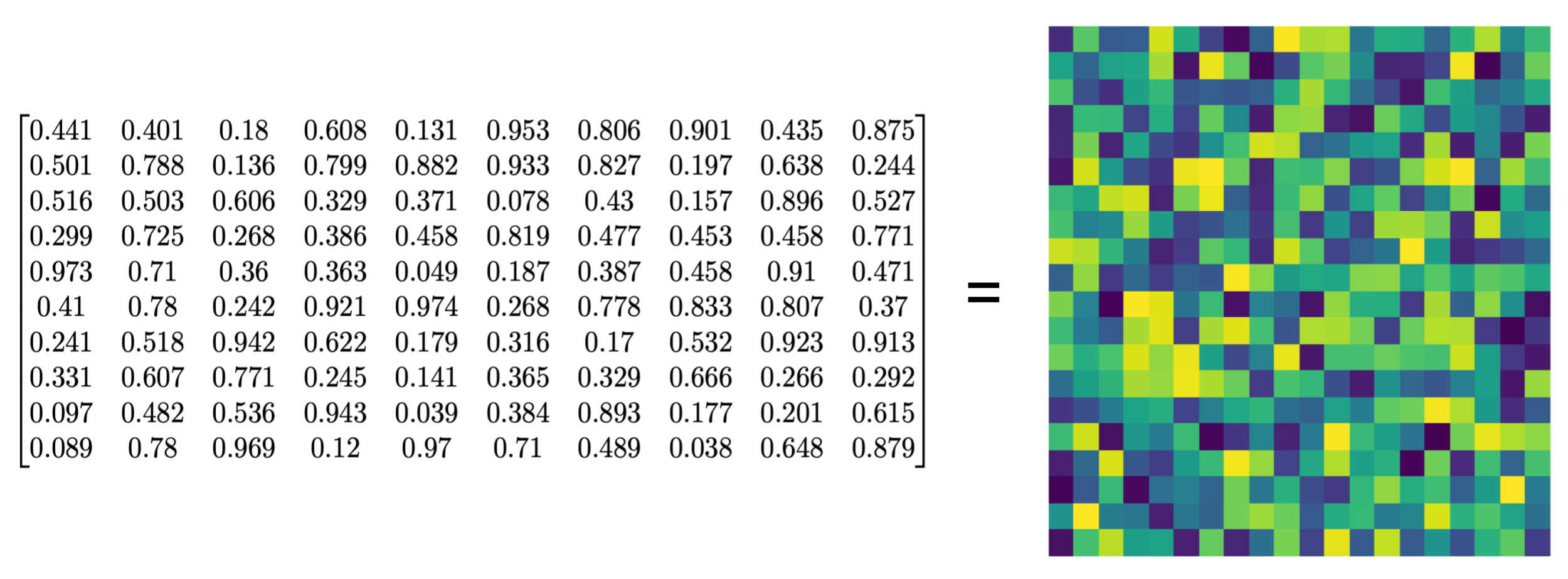
You are likely looking at superposition!
As hypothesized by
In a linear model, i.e., one which maps inputs to outputs with only linear functions, there are fewer parameters than the features it tries to represent, so it can only represent the top $m$ features. How then do neural networks use compression and map back to $n>m$ features using only $m$ parameters? The answer is non-linearity. Clearly, the activation function is key to understanding how superposition occurs - unexplored by other work in the field.
But why do we care about Superposition? Why spend time studying this?
While it may seem tangential, Superposition sheds important insights on Large Language Models (LLMs)! While LLMs are billions of parameters large, this is still not enough for a one-to-one mapping to “features” on the internet. Therefore LLMs also MUST exhibit superposition to learn. We focus our current work on the $\textit{bottleneck superposition}$ regime, but

Previous research, as detailed in
So you train a neural network - what happens at the neuron level? There are three possibilities. As the network trains each neuron has three choices:
- The neuron chooses not to encode the “features”
- The neuron chooses to dedicate itself to one feature
- The neuron chooses to encode multiple features
(We anthropomorphize - The neuron doesn’t choose to do anything - there is no free will - you are born into a loss landscape and an optimizer telling you what to do.)
In linear models, each neuron is limited to representing only the most significant features (2), discarding others (1). Conversely, superposition, enabled by non-linear activation functions, adopts a more inclusive approach (3), trying to encode multiple features per neuron and learning efficient representational shortcuts.
While ReLU bears similarity to the Gaussian Error Linear Unit (GeLU) used in modern GPT architectures, a deeper understanding of how different nonlinear activations impact superposition can provide crucial insights. Such understanding is key to unraveling the complex mechanisms through which neural networks utilize non-linearities, a cornerstone in the broader narrative of neural network interpretability.
Monosemanticity and Polysemanticity
To connect to existing literature (2) and (3) above are given the names monosemanticity and polysemanticity. We will also follow this notation going forward.
To describe further, the idea of superposition in neural networks leads us to two distinct types of neuron behaviors: monosemanticity and polysemanticity.
Monosemantic neurons are those that specialize in a single, distinct feature, acting as dedicated detectors. This characteristic is often observed in the intermediate layers of architectures like Convolutional Neural Networks (CNNs), where neurons become adept at recognizing specific patterns, such as curves or colors. Polysemantic neurons do not align with just one feature but engage with multiple features simultaneously, offering a broader and more nuanced understanding of the data. This trait is essential for handling complex, high-dimensional datasets but comes at the cost of reduced interpretability.
Motivation and Notation
Our work extends the work done in
Problem Specification
The models in this experiment will be learning how to replicate a length-$n$ vector of inputs in the range $[0, 1]$ with a compression to a length-$m$ embedding (where $n>m$). The model will then use the length-$m$ embedding to recreate the length-$n$ input, using a non-linear activation function to allow for superposition.
We will run two variations of the experiment. One variation of the experiment will involve compressing inputs of size $n=10$ to an embedding of size $m=5$. This experiment aims to see how superposition occurs across many features which are encoded in a bottleneck with half the number of spots as there are features. The second variation of the experiment will involve compressing inputs of size $n=2$ to an embedding of size $m=1$. This experiment aims to understand precisely how the model encodes the second “extra” feature in a variety of settings.
To set up this experiment, we need to create a dataset that allows for superposition to occur and that also allows for interpretability of the superposition. To motivate this further, we begin with a careful discussion of features.
Features
Features are the salient “things” that a neural network learns to differentiate inputs
Technically, features are the properties which neural networks try to extract from data during learning to compress inputs to useful representations during inference. Although features can map to human-understandable concepts (e.g., dog ears), they can also represent properties of the data that are not immediately apparent to the human brain. To experiment with superposition, we need to encode features in a way that we can understand. In other words, we do not want our experimental model to learn features that we are unaware of. This would make it hard for us to interpret how the model maps features in the data to embeddings within its parameters, consequently obscuring how superposition works. To this aim, we must generate features within the training set for our model which are simple and understandable to us a priori. Similar to
Here we define two important augmentations that we used in the dataset to simulate real-world features: sparsity and importance.
Sparsity
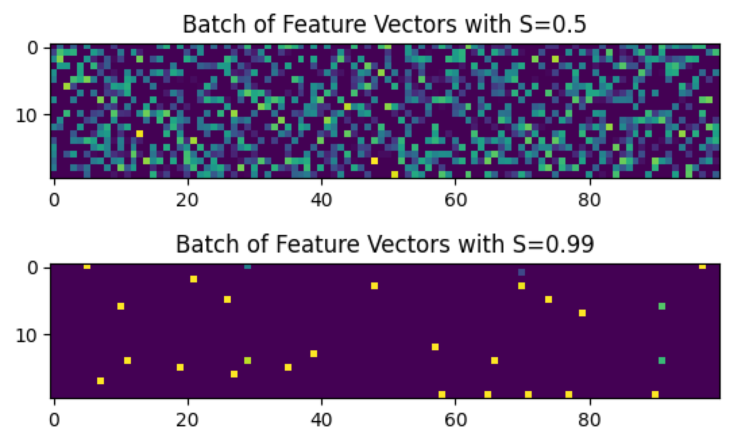
Sparsity is a measure of how often a specific feature is present in a dataset. A feature is characterized as “sparse” if it only appears in a small fraction of the inputs to the model. Similarly, features that are “dense” appear in many of the inputs. We will also use the term ‘density’, which is the complement of sparsity, defined as $1-S$.
Specifically, a feature with a sparsity of $S \in [0, 1]$ has a probability $S$ of being expressed in any given input. If we have $S=0$, this means that the feature is expressed in every input, whereas if we have $S=0.5$, this means that the feature is expected to be expressed in about half of the inputs.
In our experiment, we train models at different sparsities to capture how sparsity affects superposition.
Importance
Not all features are created equal!
Some features are more useful than others in determining relevant information about inputs. For instance, when building a dog detector - capturing features related to dogs’ faces are extremely important! A model would need to pick up salient features of dogs, perhaps floppy ears and snouts. Other features, like the grass a dog is sitting on or a frisbee in a dog’s mouth, may not be as useful for detecting a dog. The varying degrees of usefulness among features are encapsulated in the concept of “importance”.
In the context of feature detection by a neural network, importance plays a role in modulating which features are encoded within the embedded layers of the network. In the context of the superposition hypothesis, if one feature has more importance than another feature, then it would be inefficient for the network to map both features equally within the embedding; allocating more weight to the feature with greater importance would be more valuable to the network in minimizing error.
In our experiment, we give each input feature a different importance to allow the models to differentiate between them. We will examine when and how the model justifies mapping multiple features of differing importances to the same neuron, i.e., we will observe the superposition of features with differing importances.
Dataset
To run this experiment, we will synthetically generate data that has desired sparsity and importance properties.
Each input $x$ will be a vector of length $n$. Each element $x_i$ in the vector will be drawn independently from the other elements in the uniform range $[0, 1]$. As discussed before, we can now synonymously refer to each of these elements as features, given their independent generation. (We will refer to them as features from this point onwards.)
Each feature $x_i$ in the vector has a relative importance to each of the other features $x_{j\ne i}$. The importance of feature $x_i$ is $I_i = r_I^i$ where $r_I\in(0, 1)$ is a constant describing the relative decay of importance between neighboring features. This attribute of the data will be implemented in the loss function (see below for more details).
We will train separate models for each of the varying levels of sparsity. For an input $x$ with sparsity $S$, each feature $x_i$ will take on its “true” value, a uniformly distributed number, with a probability of $1-S$ and will otherwise be set to 0 with a probability of $S$.
Below is a visualization of two batches of inputs with respective sparsities $S=0.5$ and $S=0.99$.
Network
Below are the architectures of the base (linear) and experimental (non-linear) models that we are using in this experiment. Of particular note is the activation function $\mathbb{f}$, which we will substitute using the aforementioned activation functions.
| Linear Model | Activation ( $\mathbb{f}$ ) Output Model |
|---|---|
| \(h = Wx\) | \(h = Wx\) |
| \(x' = W^T h + b\) | \(x' = f(W^T h + b)\) |
| \(x' = W^T Wx + b\) | \(x' = f(W^T Wx + b)\) |
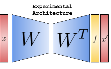
We create an autoencoder - compressing down to induce polysemanticity. This maps $x$ to a direction in a lower-dimensional space, represented by \(h = Wx\). Each column of $W$ corresponds to a lower-dimensional representation of a feature in $x$. To reconstruct the original vector, $W^T$ is used, ensuring clear feature representation correspondence. This structure results in a symmetric matrix $W^TW$ and allows for clear visualization of the weights. They visually allow for the determination of the presence of superposition.
Loss
Sparsity, Importance and Our Network come together in the following loss function:
\[L = \sum_{i} \sum_{x} I_{i}(x_{i} - x'_{i})^{2}\]Motivated by
Results
Below we present each activation function, along with plots depicting how training results in superposition at varying degrees of sparsity.
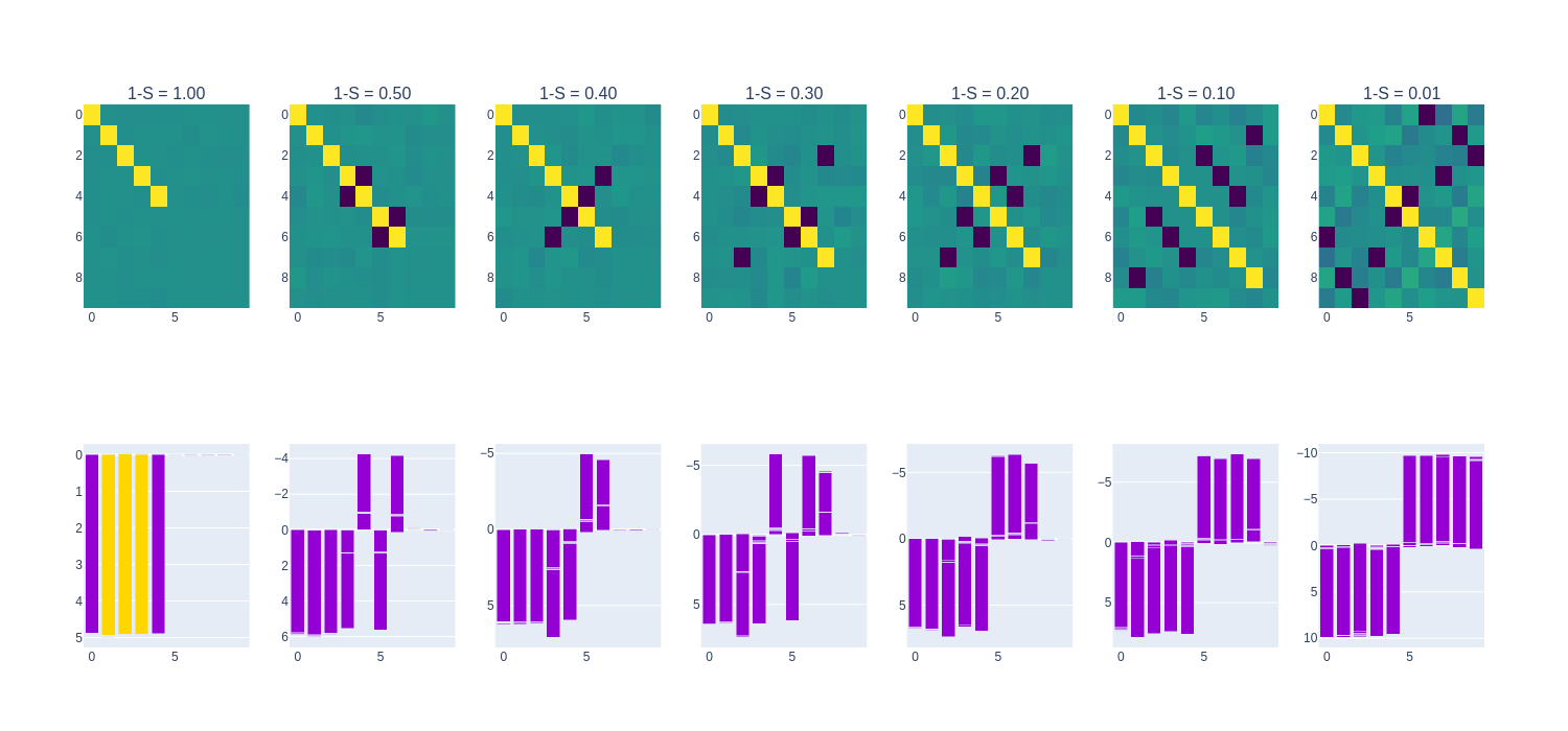
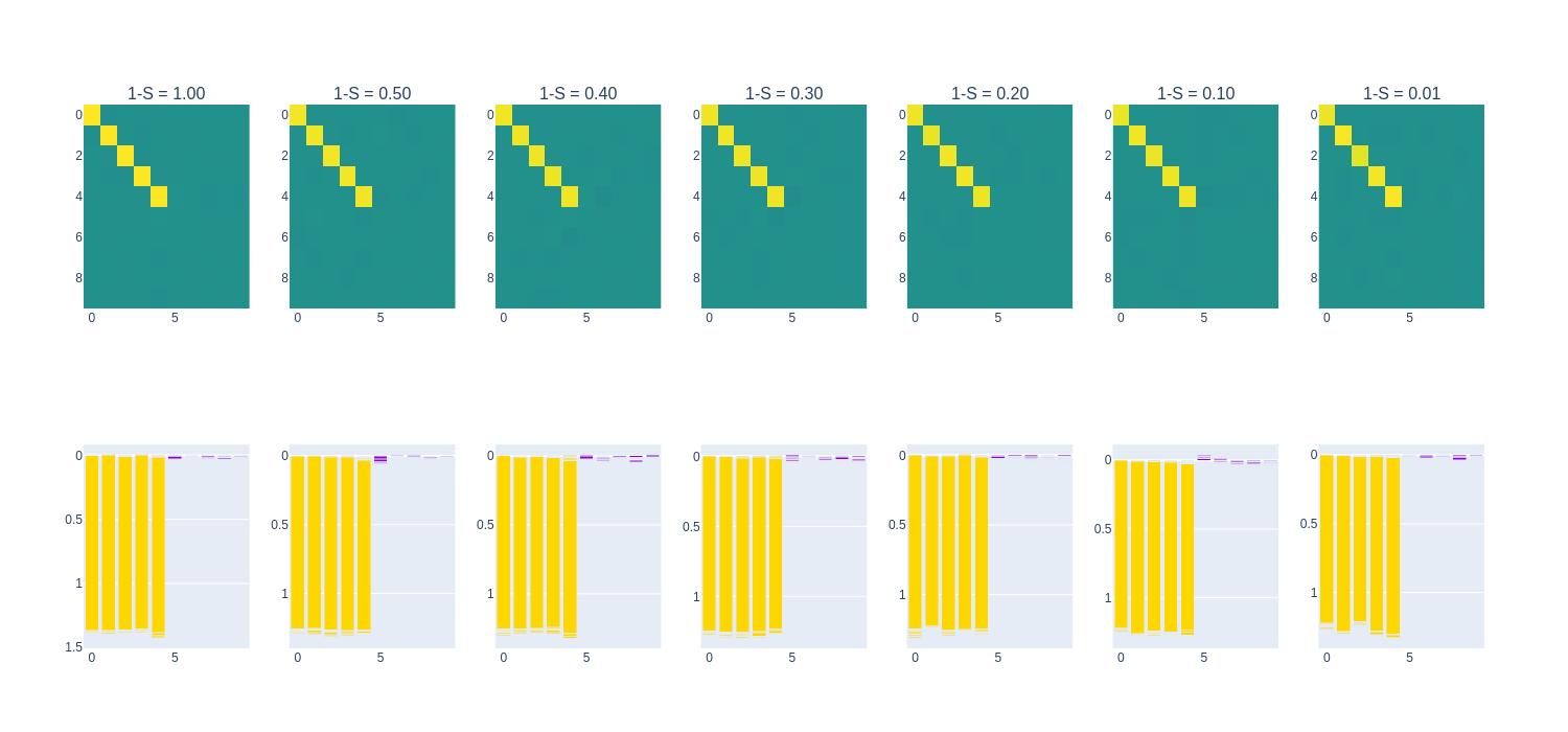
For the $n=10, m=5$ experiment, we show the $W^TW$ matrix and neuron feature distribution at varying degrees of sparsity. The $W^TW$ matrix reveals which features are prioritized (shown by the diagonal terms) and any polysemanticity that occurs (shown by the off-diagonal terms). The neuron feature distribution shows how each of the $m=10$ features are mapped to each of the $n=5$ embedding dimensions. This can aid in understanding under what conditions polysemanticity arises and how it occurs under each condition of sparsity.
For the $n=2, m=1$ experiment, we show a phase diagram. This phase diagram shows how the second “extra” feature of the length-2 input vector is encoded. There are three options: not encoded at all (only the first feature is encoded), encoded in superposition with the first feature, and encoded as the only feature (the first feature is not encoded).
ReLU
The ReLU (Rectified Linear Units) activation function is a piecewise-linear function, a simple non-linearity that allows models to use superposition of features. ReLU was the only activation function used in
The following are the $W^TW$ matrices and feature-neuron mappings:
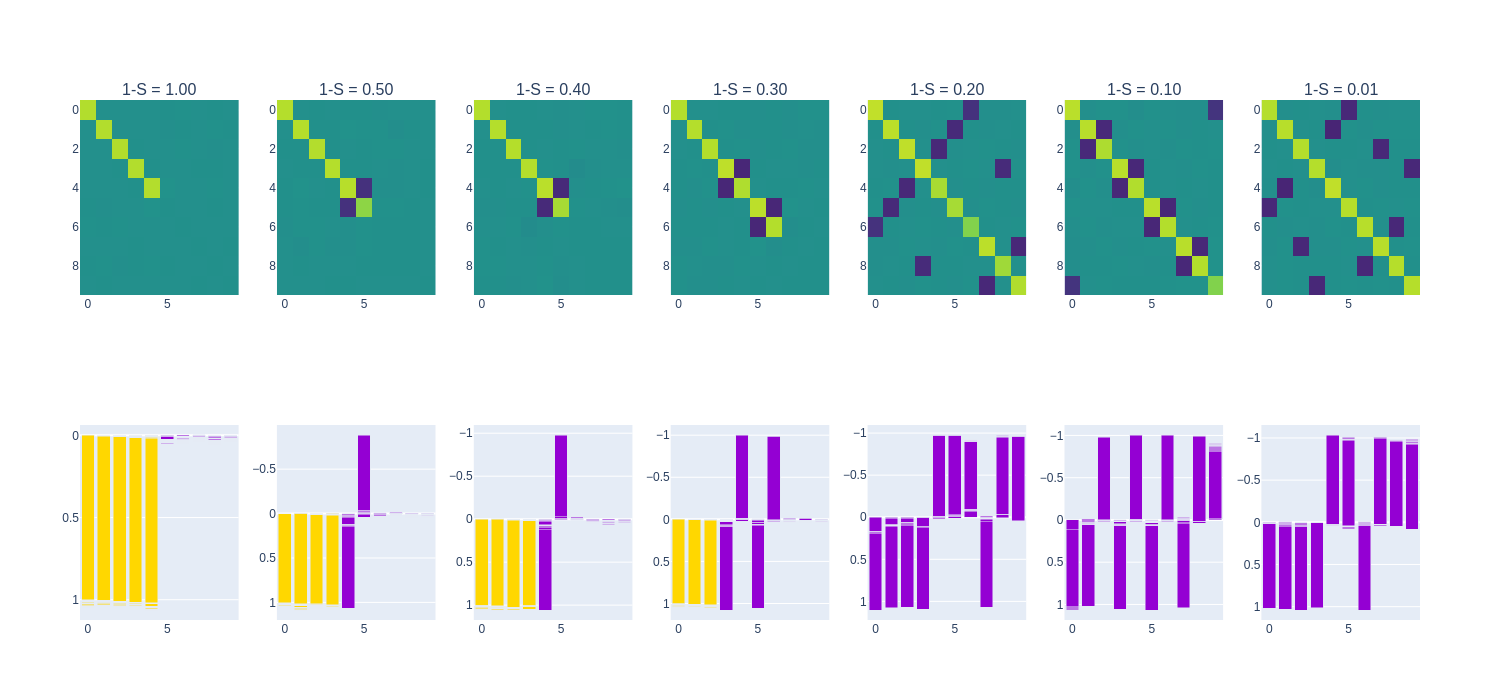
As per the results in
The following is the phase diagram of the ReLU models:
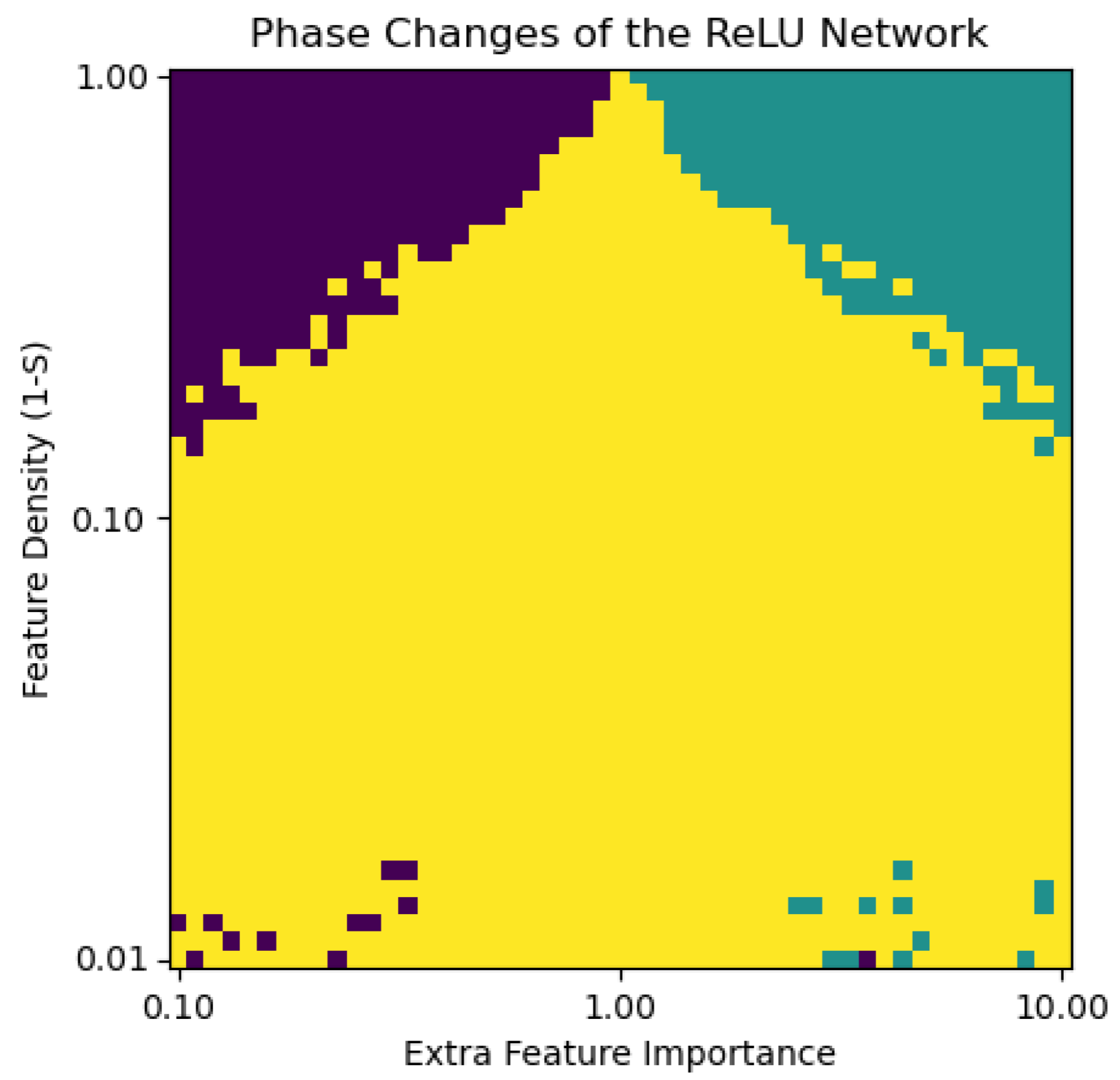

In regimes of high sparsity (i.e., below $1-S=0.1$ on the phase diagram above) the ReLU models are highly polysemantic for all relative feature importances, reflecting an inability to encode features with a sparse signal. In regimes of low sparsity, the model generally embeds the more important of the two features. This result mirrors the phase diagram in
GeLU/SiLU
The GeLU (Gaussian Error Linear Units) and SiLU (Sigmoid Linear Units) activation functions are very similar to one another, and as a result produced very similar experimental results. Both functions are akin to a “smoothed out” version of the ReLU function, i.e., they have no discontinuities. The GeLU has recently been popularized as the activation function of choice in many transformers, including BERT
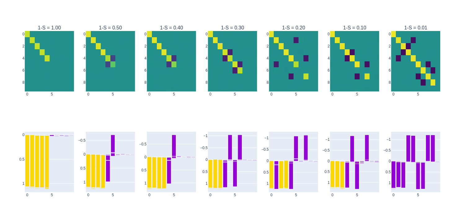
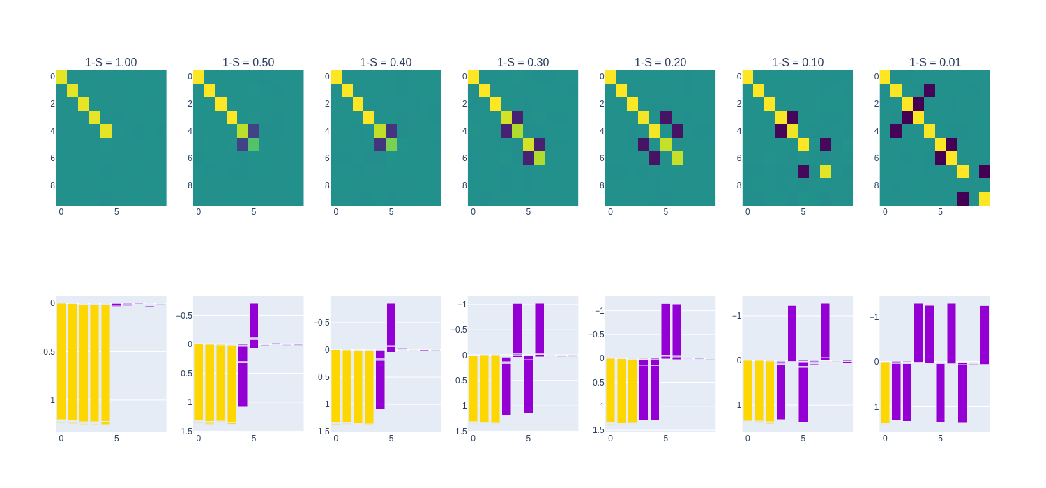
The GeLU and SiLU models exhibit similar kinds of superposition in their weight matrices. With increasing sparsity, superposition of features does happen, but it is more “strict” than the ReLU model, generally mapping at most two features to any single neuron. In each of the polysemantic neurons, though, there is one feature that dominates, suggesting that these activation functions enforce sparsity in their activations. There are also many antipodal pairs of features within these models, reiterating the behavior that exists in the ReLU models (also found in
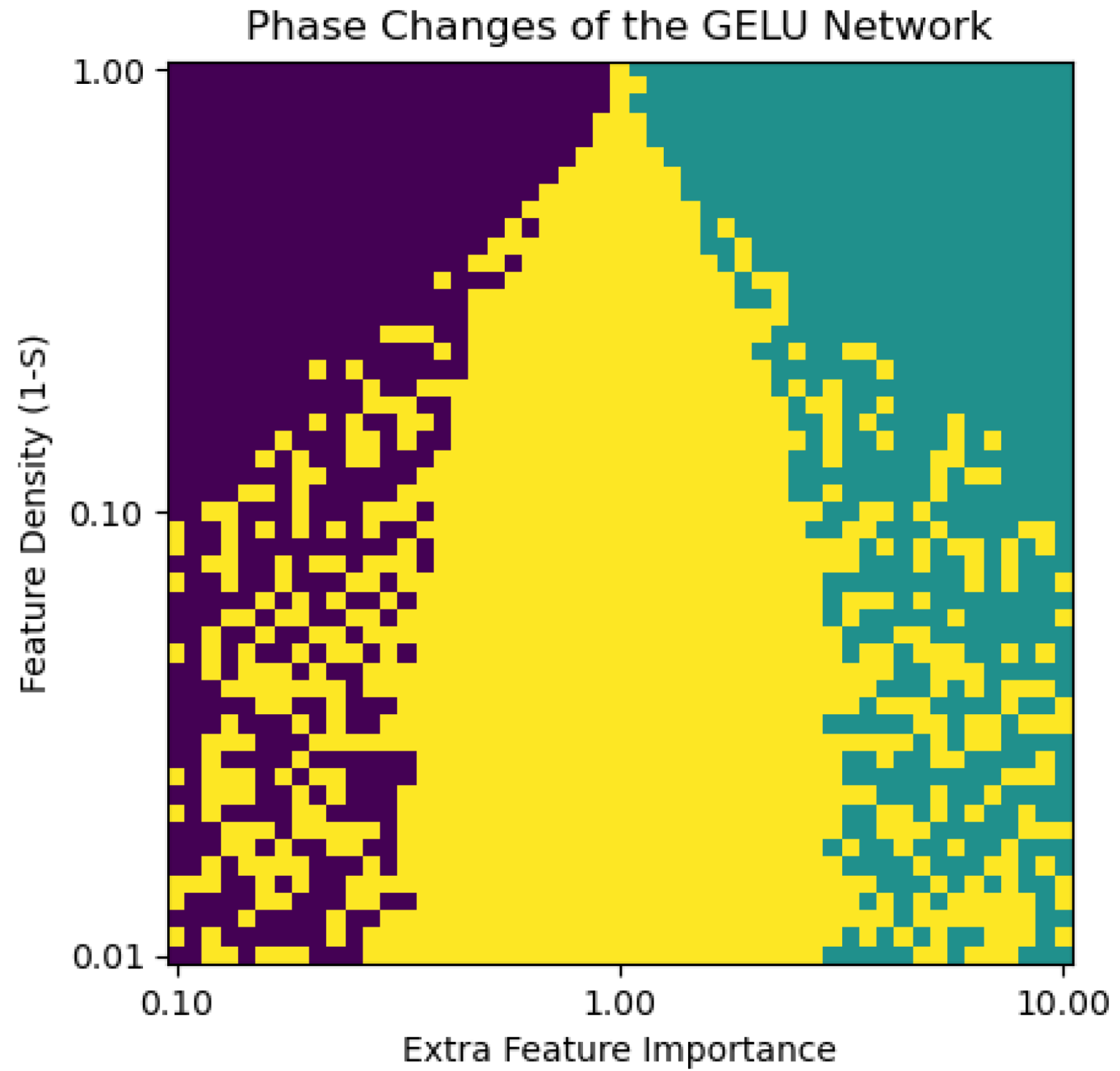
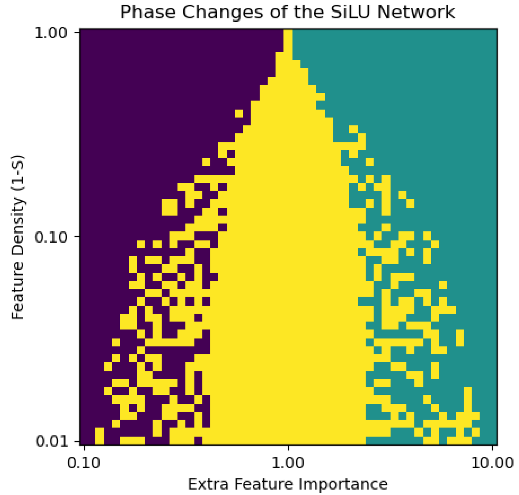

The above phase diagrams of the GeLU and SiLU models show a marked difference from that of the ReLU model (earlier), despite the similar shapes of these three activation functions. The GeLU and SiLU models exhibit significant monosemanticity at high degrees of sparsity, unlike the ReLU, which results in near-complete polysemanticity for sparsities higher than $S=0.9$. This differnce may reflect SiLU’s and GeLU’s better fit as an activation for picking up the signal in sparse feature representations, making the case for GeLU and SiLU as more interpretable activation functions within larger models.
Sigmoid
The Sigmoid function is a smooth activation function with an output range of $(0, 1)$. This maps directly to the desired range of values that the model is trying to replicate.
The Sigmoid model exhibits superposition in all neurons as soon as the sparsity is non-zero, as can be seen from the “speckling” of non-zero off-diagonal terms in $W^T W$. This is a difference from the ReLU/GeLU/SiLU models, for which the superposition “leaks” into the least significant encoded features at low, non-zero sparsities and eventually affects all features at higher sparsities. This low-sparsity superposition may occur because the Sigmoid function strictly maps to $(0, 1)$, with increasingly large pre-activation inputs necessary to map to values close to 0 and 1. As such, the model may be “speckling” the off-diagonal values in an attempt to “reach” these inputs which are close to 0 and 1.
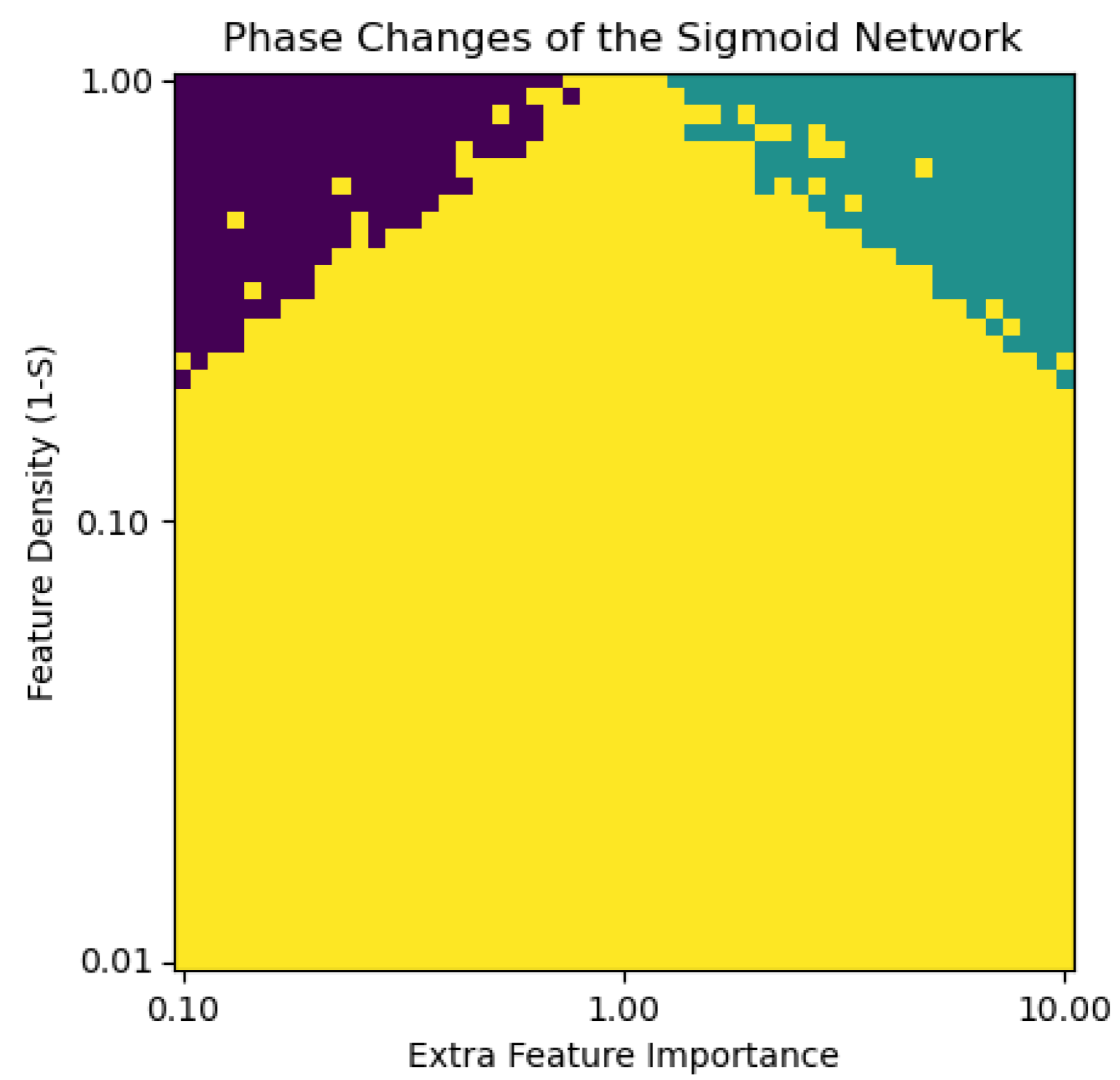

Despite differences in the occurrence of polysemanticity, the ReLU and Sigmoid models exhibit very similar phase diagrams, reflecting an inability to encode multiple features at sparsities above $S=0.9$ (i.e., below $1-S=0.1$ on the phase diagram). As discussed above, this may be caused by the vanilla sigmoid activation’s inability to “reach” target values close to 0 or 1.
Tanh
The Tanh function is another smooth activation function, but it results in significantly different behavior from the Sigmoid (despite being a linear mapping of the Sigmoid).
With the Tanh activation function, the models prioritize the most important features regardless of sparsity. This behavior is possibly attributed to the range that the Tanh function maps to $(-1, 1)$, while the target range of input values in this experiment are $[0, 1]$. This behavior is similar to that of a linear model (i.e., no activation function) which exhibits no capability to use superposition, but the phase diagram reveals subtle differences from the linear model results.
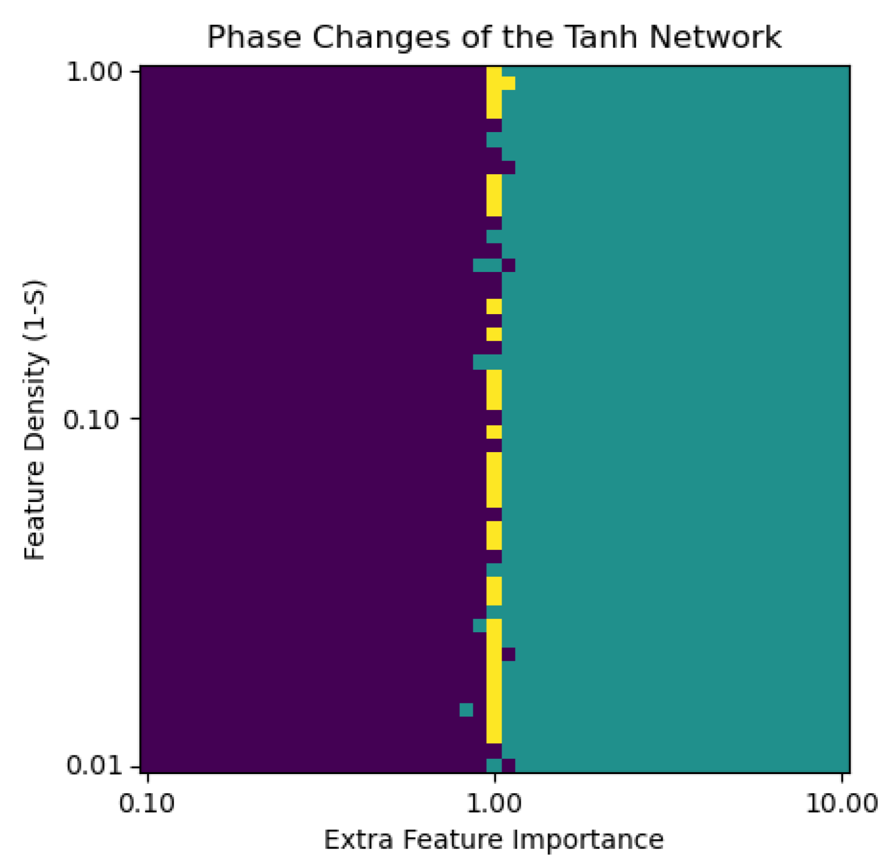

Although nearly performing as the linear model would, only encoding the most important feature, there is some difference to the linear model along the boundary between features, as can be seen around the importance of 1. This reflects the model’s ability to use non-linearity to perform superposition.
A Note on Sigmoid and Tanh
Despite similarities in the S-like curvature of the Sigmoid and Tanh activation functions, the Sigmoid model exhibits superposition, whereas the Tanh model exhibits nearly zero superposition. A key difference between the two functions is the fact that the Sigmoid function maps inputs to a range of $(0, 1)$, while the Tanh function maps inputs to a range of $(-1, 1)$. This difference is significant in our experiment, as our experiment uses models to recreate random vectors with elements in the range $[0, 1]$. The range of the Sigmoid function matches this range, while the range of the Tanh function which matches this range only occurs for non-negative inputs to the Tanh function. In other words, the $(-\infty, 0)$ input domain (which maps to the range $(-1, 0)$) of the Tanh function remains useless for prediction of values which should be in the range $[0, 1]$. Therefore, the tanh function empirically acts like a linear function (i.e., no activation layer).
SoLU
The SoLU (Softmax Linear Units) activation function is based on the work from
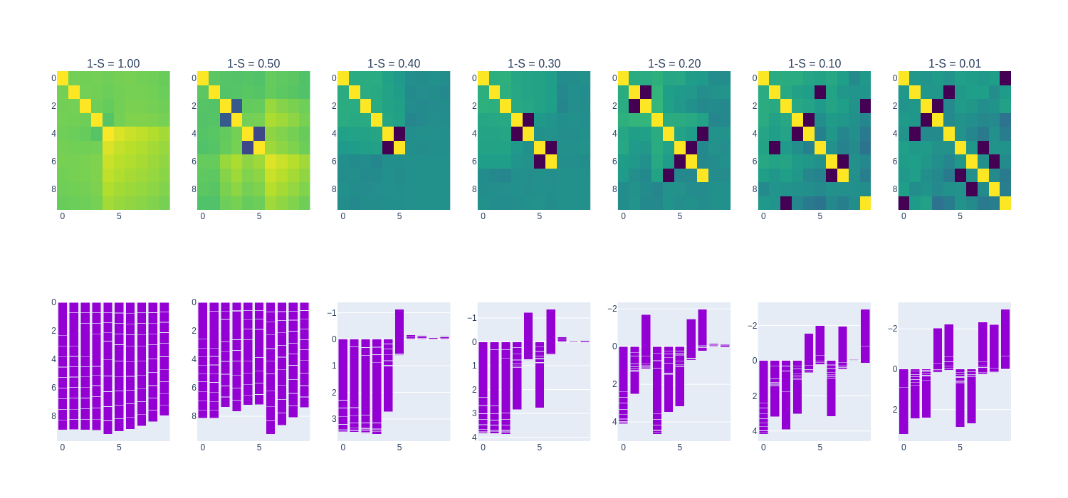
In our experiment, the SoLU model results in non-zero superposition of all features with all degrees of sparsity. This may be attributed to the way that the SoLU “forces” activations to be sparse, i.e., the activations result in a “winner-takes-all” behavior due to the way that the Softmax function works. This is not a useful property for prediction of a vector of independently-drawn values, as the input vectors are unlikely to be peaky, i.e., the SoLU does not quite fit the purposes of its task.
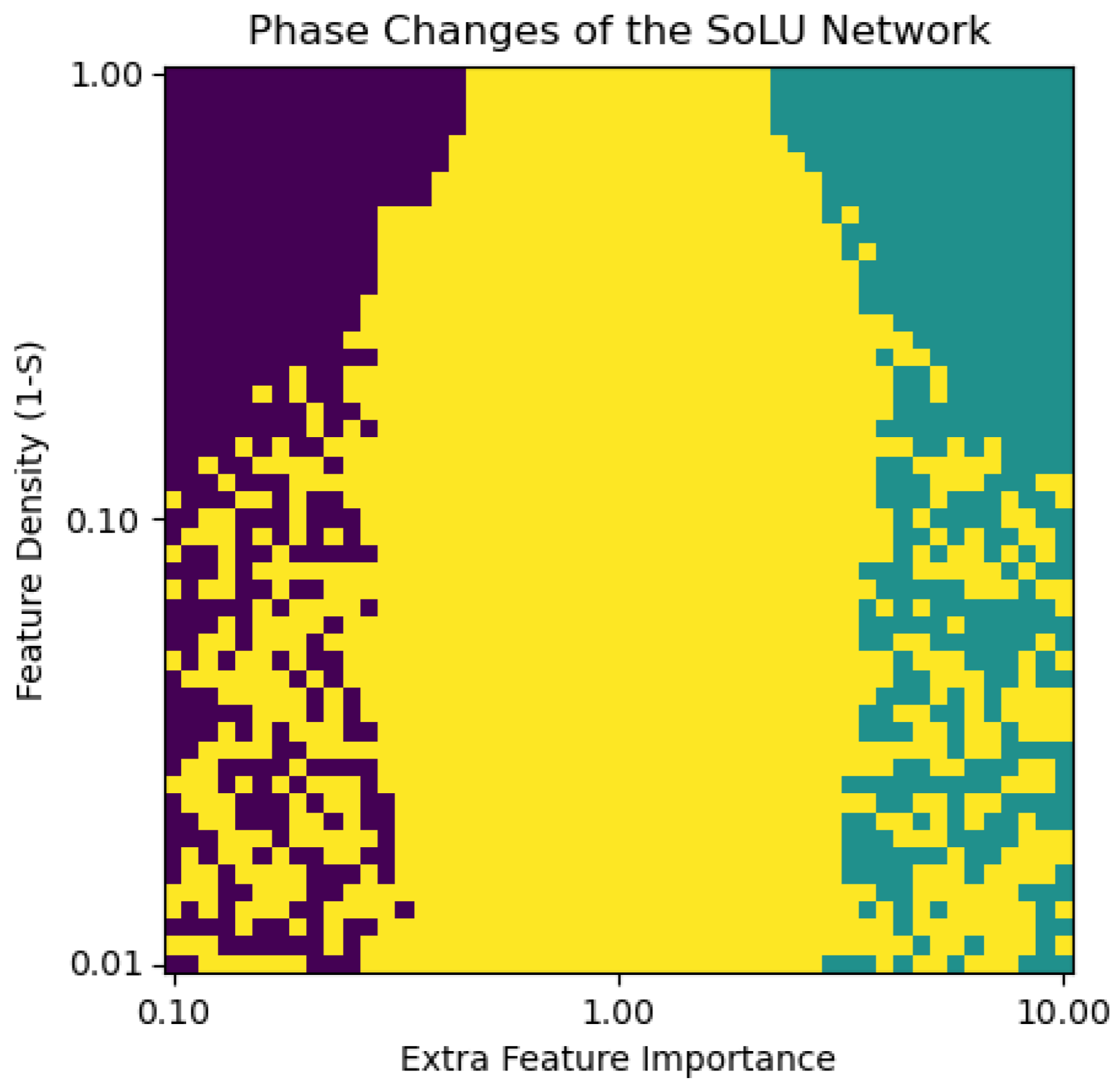

As seen in the heatmap plot above, the SoLU activation results in very polysemantic behavior. This function is not precisely fit for its task of recreating given vectors and likely results in using polysemanticity to attempt to pass information about inputs forward. Curiously, the SoLU models have preference for the more important feature in the low sparsity regime.
Bringing Them All Together
The diagram above depicts a variation on the two experiments explained thus far. In this experiment $n=200$ features were compressed to $m=20$ features and the loss function was tweaked to give uniform importance $I_i = 1$ to all features. This was done to determine how each activation functions compresses features in different sparsity regimes without the influence of feature importance.
On the y axis, the plot depicts a metric (dimensions per feature) that measures the number of dimensions a model dedicates to each feature. In other words, a point with a y-value near 1 represents a model that dedicates one dimension of its embedding space to one feature, whereas a point with a y-value near 0.25 represents a model that represents four features at each dimension.
The plots are generally consistent with the analysis from the previous experiments. Many of the activations result in superposition in the low-density/high-sparsity regime, and increases in sparsity result in increases in the polysemanticity of the model (i.e., the dimensions per feature decrease). Consistent with the other experiments, SiLU and GELU perform very similarly. The Sigmoid and SoLU activations pack nearly 20 features per dimension at high sparsities. The Tanh activation exhibits behavior similar to the linear model, neatly packing one dimension with one feature, a result that is mirrored in the previous experiments. Similar to the results in
Conclusion
Our investigation into the effects of various activation functions reveals that significant changes occur in model behavior depending on the chosen function. This finding underscores the ability to modulate the degree of superposition through the selection of activation functions, highlighting yet unexplored degrees of freedom in model design. This line of inquiry goes seamlessly with considerations of how neural networks are initialized and trained, suggesting these as promising future research directions.
Our work is limited by the breadth of activation functions that we tested, though. Further iterations on each of the activation functions (e.g., tweaking the Sigmoid function to map to the range $(-\epsilon, 1+\epsilon)$) could prove fruitful in getting better performance from the models. Furthermore, while writing this blog,
Pursuing enhanced interpretability, however, does not come without its challenges. Specifically, striving for transparency and understandability in neural network models raises concerns about the potential for deception. Despite these challenges, our work aims to develop neural network models that are more interpretable, transparent, and secure.