Guided Transfer Learning and Learning How to Learn: When Is It Useful?
For downstream tasks that involve extreme few-shot learning, it's often not enough to predispose a model with only general knowledge using traditional pre-training. In this blog, we explore the nuances and potential applications of Guided Transfer Learning, a meta-learning approach that allows a model to learn inductive biases on top of general knowledge during pre-training.
Introduction/Motivation: Never Enough Data
If we take a step back and reflect upon the current state of AI, especially in domains like computer vision and NLP, it appears that the gap between machine and human intelligence is rapidly narrowing. In fact, if we only consider aspects such as the predictive accuracy of discriminatory models and the sensibility of outputs by generative models, it may seem that this gap is almost trivial or even nonexistent for many tasks. However, every time we submit a training script and leave for the next few hours (or few weeks), it becomes abundantly clear that AI is still nowhere near human intelligence because of one critical kryptonite: the amount of data needed to effectively train AI models, especially deep neural networks.
While we have tons of training data in domains such as general computer vision (e.g. ImageNet) and NLP (e.g. the entirety of the internet), other domains may not have this luxury. For example, bulk RNA-sequencing data in biomedical research is notoriously cursed with high dimensionality and extremely low sample size. Training AI models on bulk RNA-sequencing datasets often leads to severe overfitting. In order to successfully utilize AI in domains like biomedicine, the highest priority challenge that must be addressed is that of overcoming the necessity of exuberant amounts of training data.
Machine vs Human Intelligence
It often feels like the requirement of having abundant training samples has been accepted as an inevitable, undeniable truth in the AI community. But one visit to a preschool classroom is all that it takes to make you question why AI models need so much data. A human baby can learn the difference between a cat and a dog after being shown one or two examples of each, and will generally be able to identify those animals in various orientations, colors, contexts, etc. for the rest of its life. Imagine how much more preschool teachers would have to be paid if you needed to show toddlers thousands of examples (in various orientations and augmentations) just for them to learn what a giraffe is.
Fortunately, humans are very proficient at few-shot learning– being able to learn from few samples. Why isn’t AI at this level yet? Well, as intelligence researchers have discussed
Traditional Transfer Learning: Learning General Knowledge
Transfer learning has been invaluable to almost all endeavors in modern deep learning. One of the most common solutions for tasks that have too little training data is to first pre-train the model on a large general dataset in the same domain, and then finetune the pre-trained model to the more specific downstream task. For example, if we need to train a neural network to determine whether or not a patient has a rare type of cancer based on an X-ray image, we likely will not have enough data to effectively train such a model from scratch without severe overfitting. We can, however, start with a model pre-trained on a large image dataset that’s not specific to cancer (e.g. ImageNet), and if we start training from those pre-trained weights, the downstream cancer diagnostic task becomes much easier for the neural network to learn despite the small dataset size.
One way to intuitvely understand why this is the case is through the lens of “general knowledge”.
However, if transfer learning could solve all our problems, this blog post wouldn’t exist. When our downstream dataset is in the extremeties of the high dimensional, low sample size characterization (e.g. in fields like space biology research, more on this later), learning general knowledge in the form of pre-trained weights isn’t enough.
Guided Transfer Learning and Meta-learning: Learning Inductive Biases
Guided transfer learning (GTL)
GTL is a very novel method; its preprint was just released in the past few months! Hence, beyond the experiements in the original preprint, there has not been much exploration of some of its behavioral nuances and various application scenarios. So in this blog, I will be doing a few experiments that attempt to gain more insight into some of my questions that were left unanswered by the original GTL paper.
But before we get to that, let’s first get a rundown on how GTL works! The two most important concepts in GTL are scouting and guide values.
Scouting
Inductive biases, which affect what kind of functions a model can learn, are usually built into the choice of deep learning architecture, or decided by other hyperparameters we humans choose. With guided transfer learning, they can now be learned automatically during pre-training. It’s almost like the model is figuring out some of its own optimal hyperparameters for learning in a particular domain.
Sounds like magic, right? How does GTL allow a model to learn inductive biases? Well, the core behind the GTL approach is a process known as scouting, which is an alternative to traditional pre-training. The high-level idea is that it trains copies of the model, called scouts, on easier subproblems. These subproblems should be similar to the target downstream tasks, but easier so that the scouts are more likely to succesfully converge to a generalizable model. (If the scouts themselves overfit, then how can the inductive biases they learn help our downstream few-shot training not overfit?)
In the process of converging, the scouts keep track of which parameters in the model are important to keep flexible for efficient convergence and which ones aren’t. They’re basically logging their learning process.
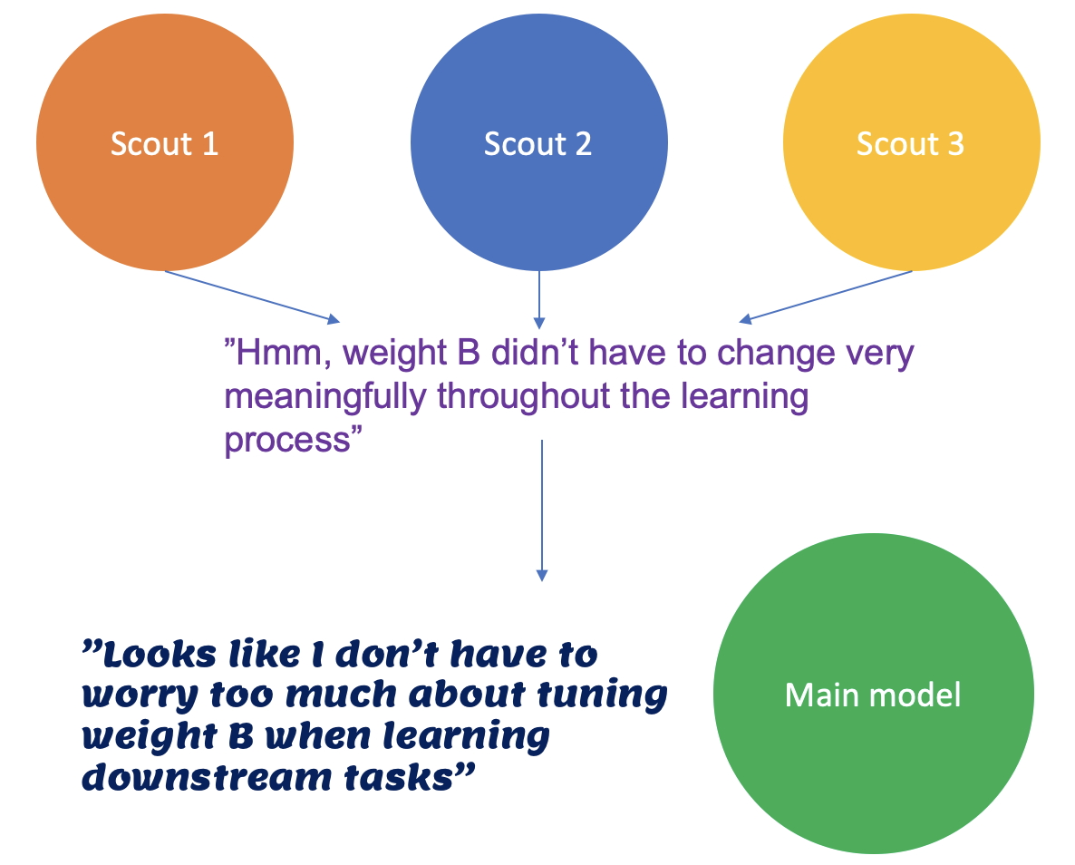
For example, if weight A increases drastically during training, it’s probably an important weight to change and we should keep it flexible. On the other hand, if weight B doesn’t change much at all or fluctuates in a very noisy manner (i.e. doesn’t change meaningfully), it is probably not as important to change.
After the scouts are finished training, the collective feedback from all the scouts is used to decide what inductive biases to impose on the main model, such that the main model can learn most efficiently for the particular domain of data and avoid wasting effort and being distracted/misguided by changing parameters that don’t really help in that domain.
Guide Values
So what do these “inductive biases” actually look like, and how do they affect future training? The inductive biases in the context of GTL come in the form of guide values. So after scouting, each parameter will not only have its usual weight value, but it will also have a guide value. During gradient decent, the normal update for a particular weight is then multiplied by its corresponding guide value. Thus, the larger the guide value, the more that parameter is allowed to change during downstream training.

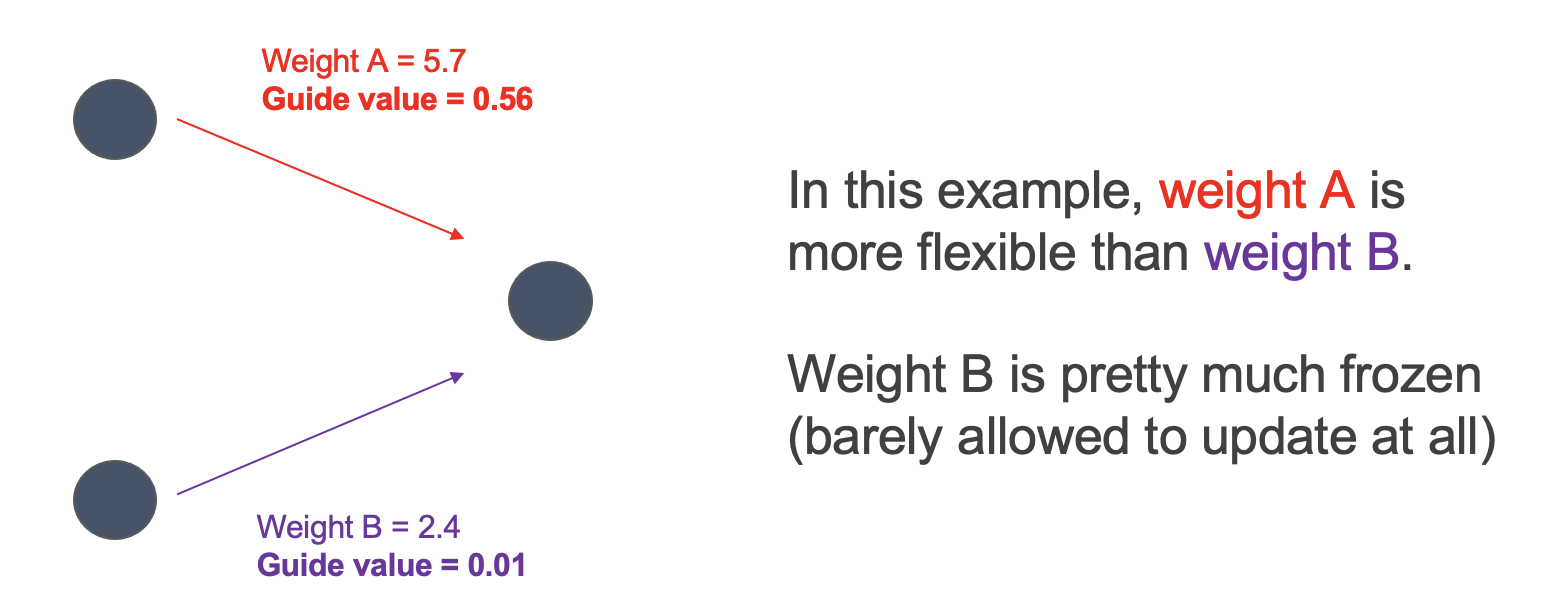
Thus, the goal of scouting is to find these optimal guide values, which will ultimately make the training process more sparse (i.e. so that only the weights that are useful to change get changed). Note that this is different from making the neural network model itself more sparse (i.e. setting weights/connections that are useless to zero).
Calculating Guide Values
So how do we actually get the guide values after training the scouts? Well, as mentioned above, we keep track of how parameters change during the scout training processes. Specifically, during the training of each scout, we log the initial value and final value (i.e. value after convergence) of each parameter in the model. Then, we calculate how much each parameter changes throughout the process of convergence via some distance metric between its initial and final value. The default used in the GTL paper was the squared distance: \((w_b - w_f)^2\), where \(w_b\) is the baseline (initial) value of the parameter \(w\), and \(w_f\) is its final value.
Now, each scout will converge differently, since they are trained on slightly different subproblems (more on this later). To have a robust estimator of how much some parameter \(w\) changes during convergence, we take the mean squared change of the parameter across all the scouts. Let’s call this value \(m_w\).
Assuming we have \(N\) scouts, this would be: \(m_w = \frac{1}{N}\sum_{i=1}^{N}(w_{b,i} - w_{f,i})^2\), where \(w_{b,i}\) and \(w_{f,i}\) are the initial and final values (respectively) of parameter \(w\) in scout \(i\).
Add on a 0-1 normalization across the \(m_w\)s of all the parameters in the model, and we have our guide values (all of which are between 0 and 1)!
Intuitively, we can see that parameters that changed a lot throughout the convergence process in the scout models are deemed “important to change during training” and are thus given higher guide values (i.e. closer to 1), allowing them to be more flexible for downstream fine-tuning.
It’s really quite an elegant and simple approach, which is the beauty of it! It’s comparably lightweight in terms of both memory and computation compared to many other popular meta-learning/few-shot learning methods.
Experiment and Results from the GTL Paper
Before we get started with some of our own experiments to explore more nuances of GTL behavior and benefits, it might be nice to establish that– Yes, it does work! Or, it at least provides very impressive benefits.
In the original GTL paper, Nikolić et al. tested how much benefit GTL would provide for few-shot learning tasks specifically in the domain of computer vision. Specifically, they tested one-shot learning capability on the Omniglot dataset.

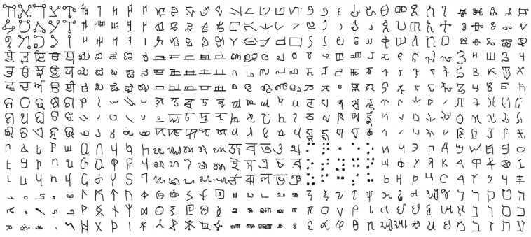
To prepare a one-shot learner for this task, Nikolić et al. pre-trained a very basic CNN using the following GTL pipeline:
- Pre-train the model traditionally on MNIST (lots of data there!). The goal here is to have the model acquire general knowledge in the form of pre-trained weights. No inductive biases yet.
- Scouting. The meat of GTL, where inductive biases are learned!
- Downstream fine-tuning and evaluation on Omniglot using the one-shot scheme described above.
The most interesting part is the second step: scouting! Remember, we have the following criteria for the scout problems:
- There needs to be multiple different scouting problems (so the we can have an ensemble of different scouts contributing to the guide value calculations, making the guide values more robust)
- The scout problems need to be easy enough so that the scouts can actually successfully learn generalizable models! Again, if the scouts themselves overfit, the guide values derived form them won’t be very helpful for downstream one-shot learning :)
- The scout problems need to be similar to the downstream task, i.e. in the same domain (in this case, computer vision) and of the same kind of problem (e.g. in this case, classification). If the scout problems are too different, why would the inductive biases be transferable?
Given these criteria, Nikolić et al. used the following scheme for generating scouting tasks:
- Create subdatasets of MNIST (termed “cousin” problems in the paper), where each subdataset/cousin contains data for only three of the digits in MNIST (120 of these cousin datasets were created in the paper).
- Train a scout on each of the cousin problems (120 scouts total).
This scheme satisfies all three criteria above. We now have multiple different scouting problems. These scouting problems are also comparatively way easier than the downstream task (there’s way more training data than Omniglot, and it’s only a 3-category classification problem). BUT, despite being easier, they’re still similar enough to the downstream task such that we can expect transferability (it’s still a handwritten character image classification task, after all).
And this worked quite spectacularly! Here are the results from their paper:
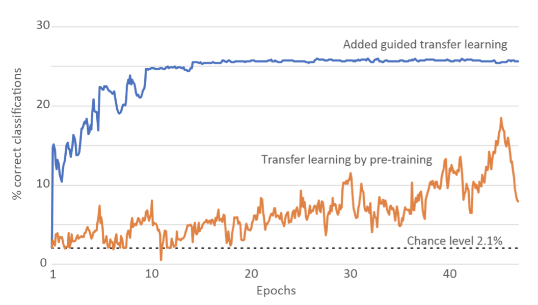
The plot on the left shows the validation curves for the downstream one-shot Omniglot task for 1) a model that was pre-trained traditionally (line in blue) and 2) the model that was pre-trained traditionally and underwent GTL scouting (line in orange). Although the GTL model was still only to get around 25% validation accuracy, that’s quite impressive for only getting one example of each character, and is a signficant improvement over the model that only experienced traditional pre-training.
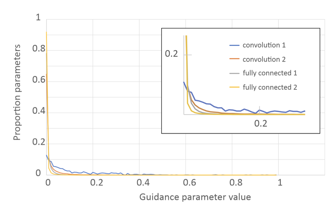
Interestingly, the plot on the right plots the distribution of guide values. We see a heavy right skew, indicating that most of the guide values are very close to 0! This means downstream fine-tuning has been made very sparse (very few parameters were allowed to change drastically), providing very strong inductive biases that heaviliy influenced how the model was allowed to learn. These inductive biases, as the results suggest, seem to be correct for the task at hand. But that shouldn’t be surprising because they were, in a way, learned.
And that is the beauty of GTL. We no longer have to “guess” what inductive biases (often in the form of architectural choices) might be appropriate for a certain domain; instead, we have these biases be “learned”!
Answering Unanswered Questions: Exploring the Nuances
Now that we see GTL does provide noticeable benefit for one-shot learning tasks based on the experiemental results from Nikolić et al., I would like to run some additional experiments of my own to explore some of the nuances of when GTL can be helpful, how we can optimize the benefit we get from using it, and how we should go about designing scout problems. These questions had not been explored in the original GTL paper, and since no other piece of literature has yet to even mention GTL, I thought I’d take the lead and try to gain some initial insight into some of these open topics :)
Experiment 1: Can GTL compensate for lack of pre-training data (not just lack of fine-tuning data)?
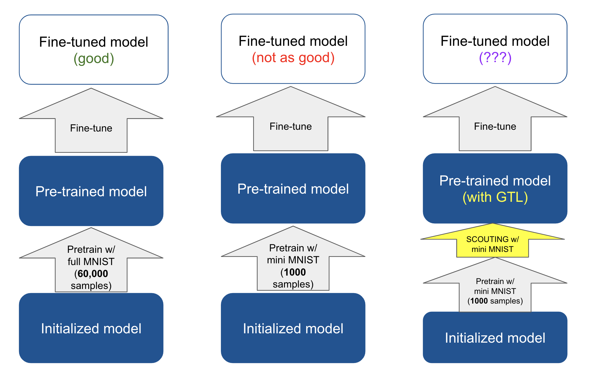
So we’ve established that GTL can aid in learning downstream tasks with few training samples, but it still requires a large amount of pre-training data (e.g. MNIST), much like traditional transfer learning. What I want to know now is: what if we don’t have that much pre-training data? In such low pre-training-data contexts, performance on downstream tasks usually suffers as a results when using traditional transfer learning. Can the addition of scouting/GTL compensate for this lack of pre-training data? That is, can a model pre-trained with a small pre-training dataset + GTL do as well as a model that’s just traditionally pre-trained on a large pre-training dataset?
Setup
To do test this, I pre-train a small CNN with a very similar GTL pipeline as the one used by Nikolić et al., but using only a mere 1000 of the full 60,000 samples from the MNIST dataset during pre-training/scouting. A significantly smaller pre-training dataset! I’ll sometimes refer to this subset of MNIST as “small MNIST”. I then evaluate the performance of this model on an Omniglot one-shot task and compare it to 1) a model that is only traditionally pre-trained on small MNIST (no GTL) and 2) a model that is traditionally pre-trained on the full 60,000-sample MNIST (also no GTL).
Downstream Task Specification
Note that the exact setup for the downstream Omniglot one-shot task used in the original GTL paper was not revealed. There are a few variations of one-shot learning setups, but the one I will be using is:
- Take a 100-cateogry subset of the full Omniglot dataset (that is, 100 unique characters)
- Train the model on one example of each unique character (i.e. 100 training samples total), and use the rest as a validation set (i.e. 1900 validation samples total)
- The task is thus a 100-way classification problem (given a handwritten image, predict which of the 100 characters it is)
Since the specification above is likely not the exact Omniglot problem setup used by Nikolić et al., and the hyperparameters they used are also not specified in the original paper, some of the baseline results I’m using do not quite match to the corresponding results in the original paper.
Results and Analysis
With that said, here are the resulting validation accuracy and loss curves for the downstream Omniglot one-shot task described above:
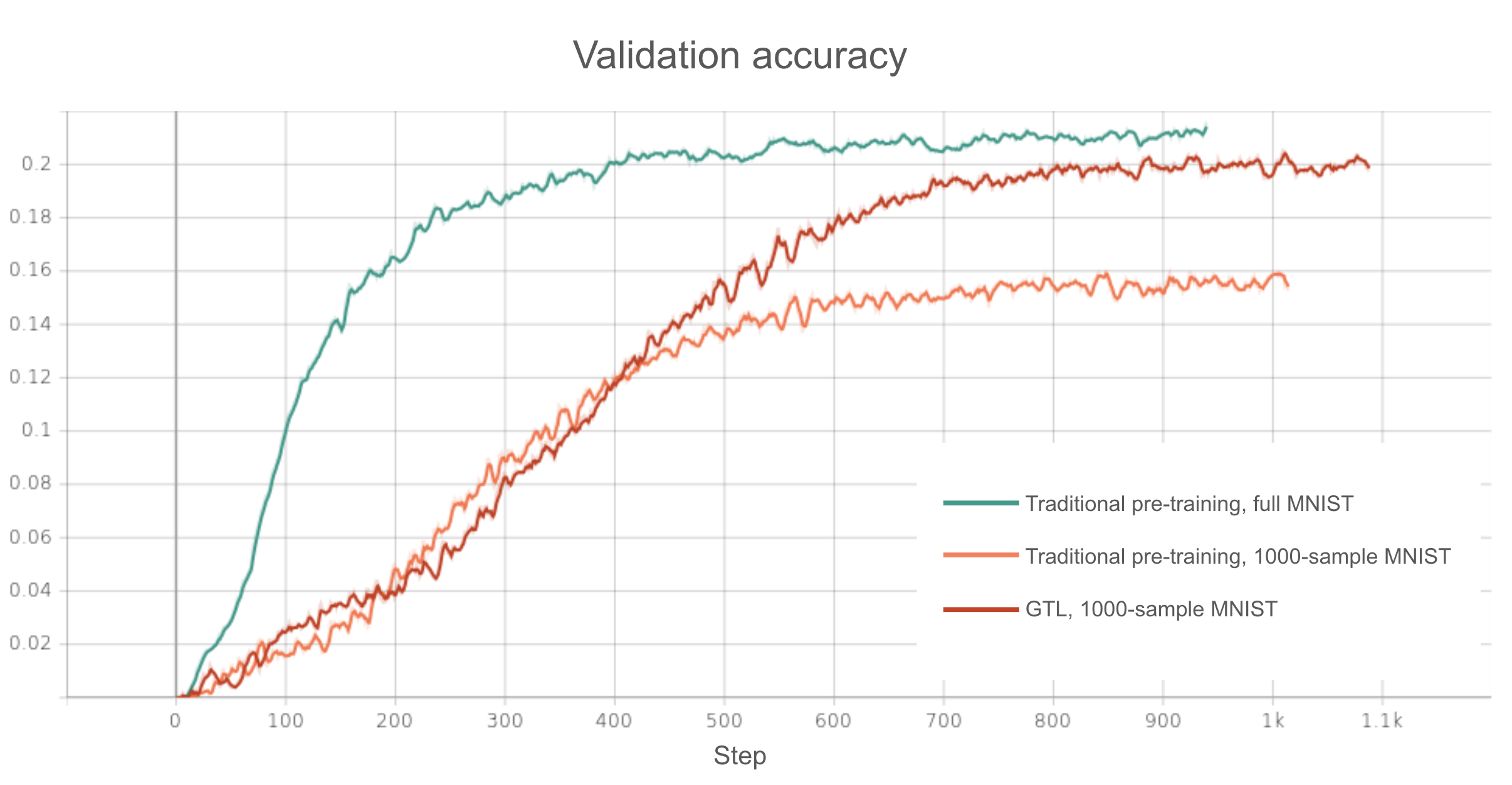
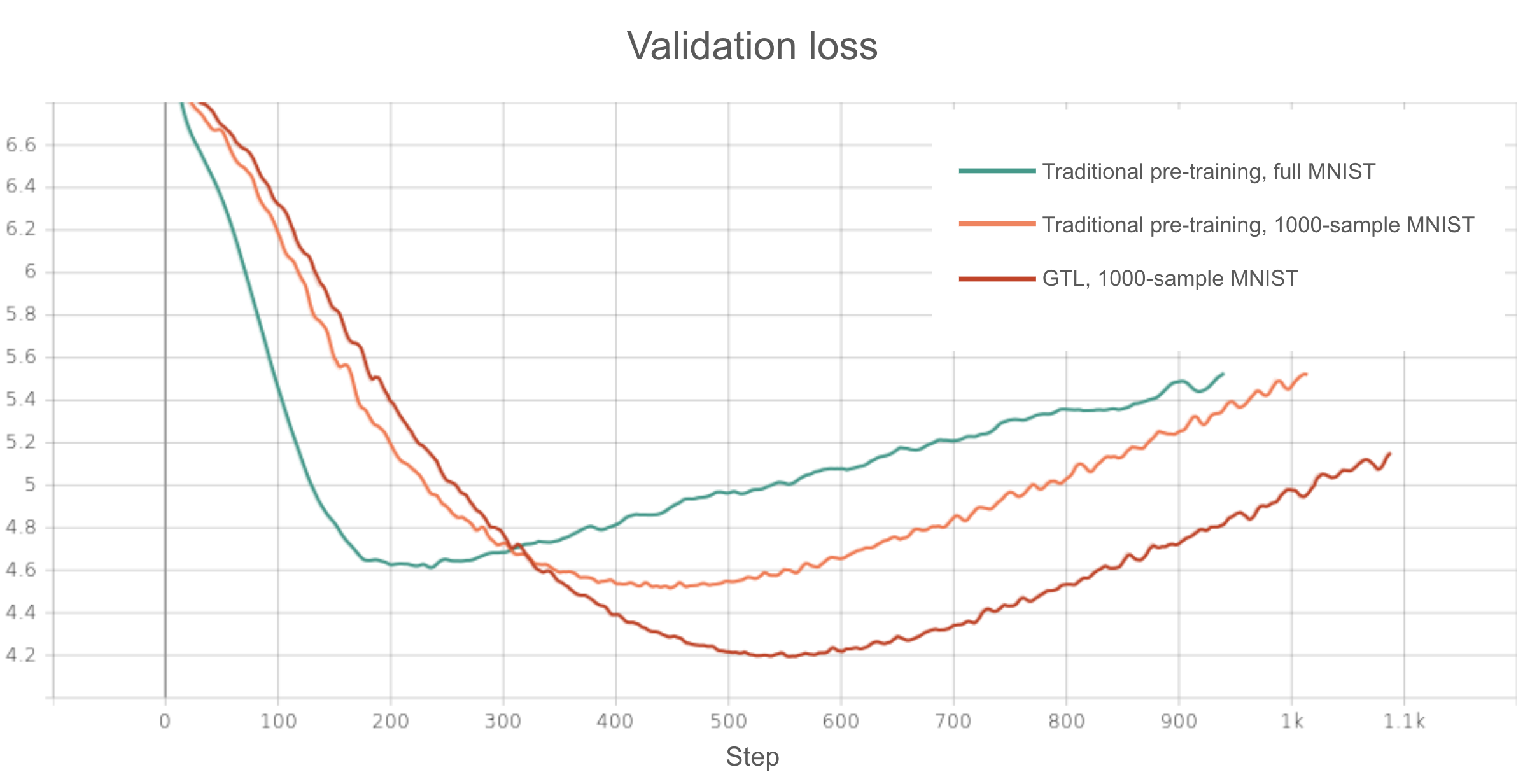
As we can see, when GTL is not used, pre-training on a 1000 sample subset of MNIST results in notably worse performance on the one-shot downtream task compared to pre-training on the full 60,000 MNIST (16% vs 21% max validation accuracy). This is as expected.
However, if we use small MNIST and add scouting/GTL (using the same scout problem set up in the original GTL paper), we see that the resulting model ends up being able to reach almost the same max validation accuracy as the model traditionally pre-trained on the full MNIST dataset (20% vs 21%).
What this suggests is that the inductive biases learned by GTL can compensate for any decrease in “general knowledge” (encoded in the form of pre-trained weights) that comes from having a smaller pre-training dataset. So not only is GTL helpful when you don’t have enough downstream data, it can also be helpful when you don’t have enough pre-training data!
Additionally, if we inspect the validation losses, we see that, depsite an apparent drop in validation accuracy, overfitting is still occuring in the shadows for all the models, as all the validation loss curves start rising after a certain point. However, the model that is pre-trained with GTL achieves the lowest validation loss of the three models before overfitting, and also starts overfitting the latest. So even though there’s no huge difference in the maximum validation accuracy achieved by the model that was pre-trained with GTL on small MNIST and the model that was traditionally pre-trained on full MNIST, the former is able to be optimized further before overfitting, suggesting that GTL with a small pre-training dataset provides a stronger “regularizing” effect than traditional transfer learning with a large pre-training dataset! This is certainly an interesting observation that could potentially have more obvious practical implications in certain scenarios, though we will not go into that further in this blog. The takeaway, however, is that GTL is, at the end of the day, really just a strong “regularizer”. If we look at how the orange and red curves look in both the accuracy and loss plots, we see the performance benefit that comes form adding GTL really just comes from the delay of overfitting. This regularization-based mechanism of performance improvement by GTL makes sense, as strong inductive biases hold the model back from learning “just anything” that fits the downstream training data.
Experiment 2: How does the design of the scouting task affect downstream performance?
Okay, it seems so far that the scouting pipeline used in the original GTL paper seems to be pretty helpful for various scenarios. But how did the authors arrive at that specific scouting task formulation? What if we used different scouting tasks than the ones they did? How does that affect GTL performance, and what might such differences (if any) imply? After all, when we leave the context of MNIST and Omniglot, we’ll have to be designing these scouting tasks on our own…
Setup
For the sake of experimental control, however, I will stick with MNIST and Omniglot for now (don’t worry, I deviate from these datasets in the next experiment). Here, I begin by testing the effects of changing how many categoriess are included the cousin subdatasets that the scouts are trained on. The original paper used 3 categories per scout dataset (i.e. a 3-way classification task). What if used 2? Or 4? And if that makes a difference, why?
In my eyes, this experiment explores how similarity between the scout tasks and the downstream task affects transferability. Specifically, because the downstream Omniglot task is a 100-way classification problem, one might expect that scout tasks that include more classification categories (and are thus more similar to the donwstream task) would result in better transferability.
To test this, I use a 5000-sample subset of MNIST for pre-training/scouting (to save computation and time). For scouting, I create 120 cousin problems, as done in the paper. But instead of sticking to 3-category cousin problems, I also try 2-category, 4-category, and 5-category problems.
Results and Analysis
Here are the results:
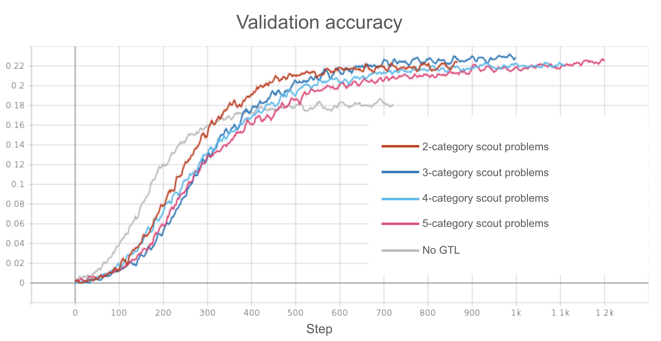
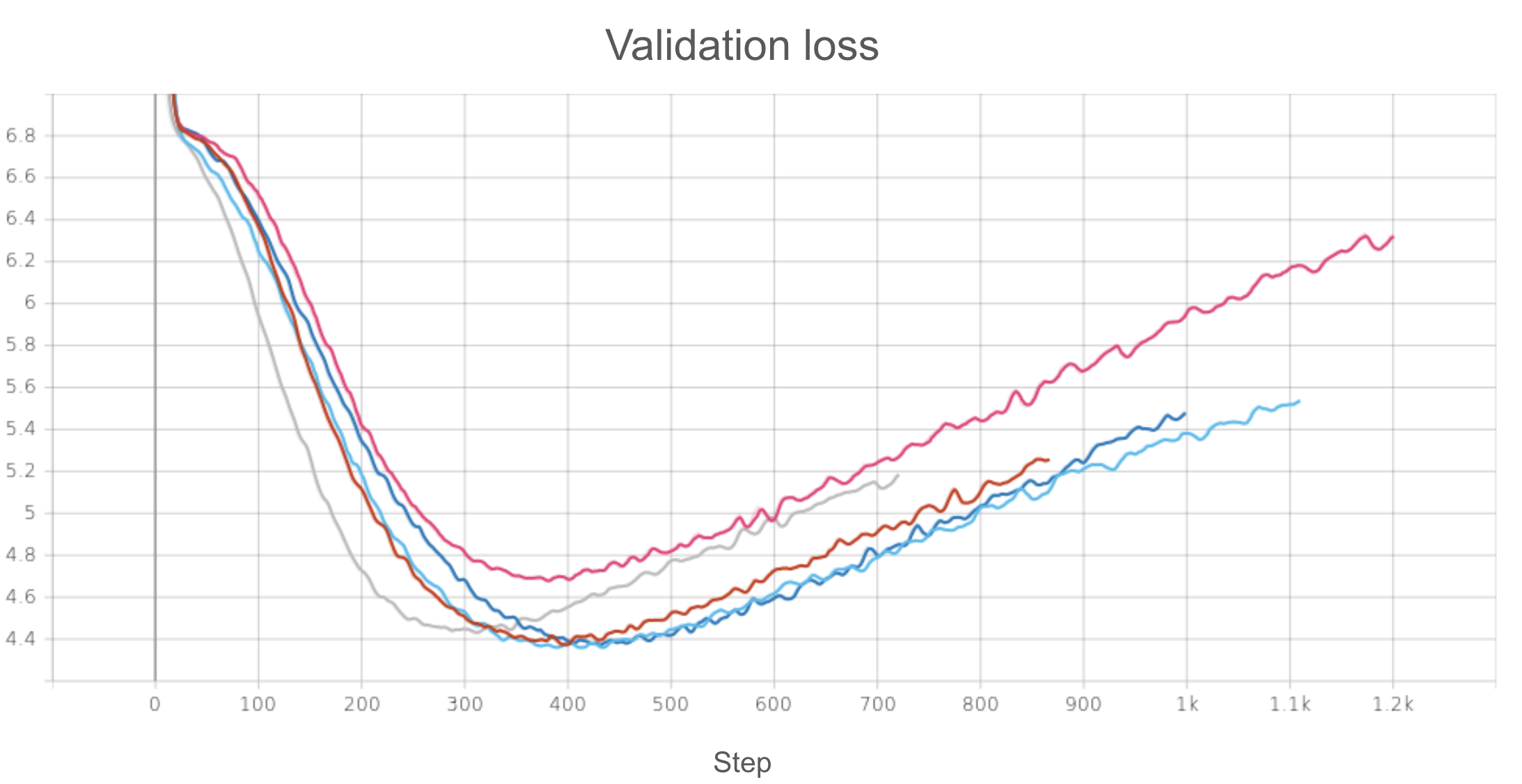
As we can see, apparently the number of categories doesn’t make too big of a difference in maximum validation accuracy! They all provide seemingly equal accuracy improvement from a baseline model pre-trained traditionally on the same 5000-sample MNIST subset. This isn’t too surprising. Compared to the 1000-way downstream classification, the difference between 2-way and 5-way classification tasks would intuitively seeem pretty negligible.
The validation loss plot tells a slightly different story, however. We see most of the models pre-trained with GTL have similar loss curves, consisting of a lower minimal loss and more resilience to overfitting compared to the baseline model. However, the model based on scouts trained on 5-category cousin problems seems to achieve the worst (highest) minimum validation loss! This seems… a bit hard to explain. Perhaps this is just due to stochasticity; after all, we see that overfitting still occurs later relative to the baseline model, suggesting there still is some resilience to overfitting.
But a perhaps more interesting explanation (that admittedly could be completely wrong) is that 5-category problems may have been too difficult of a scouting task given the smaller subset of MNIST used (since lots of categories + few training samples is a often recipe for overfitting). That is, perhaps many of the scouts themselves would have started overfitting while being trained on these subproblems, so the guide values derived from such scouts don’t end up providing robust enough inductive biases.
Again, this is just a speculation, but if it were true, this could suggest an interesting tradeoff between the easiness of the scouting tasks and their similarity to the target downstream task. Make a scouting task too easy, and it’s too different from the target downstream task, and transferability suffers as a result. Make a task too similar to the target downstream task, and it might be too difficult, causing the scouts themselves to overfit and the resulting guide values to be less useful. An intersting balance to think about and explore further.
The overarching takeaway from this experiment, however, seems to be that the exact number of categories for the scouting problems at this specific scale does not drastically affect downstream one-shot performance. Sure, I could have tried to keep increasing the number of categories, but keep in mind there’s also a bit of a tradeoff between number of categories and number of possible scouts past a certain point. For example, we would only be able to have one cousin problem with 10 categories (and it would be the whole MNIST dataset)!
Experiment 3: What about unsupervised/self-supervised settings?
Note: This particular experiment builds off of some previous work I have done outside of this class.
For the final experiment, I would like to provide a bit of my research background for context. I’m primarily intereted in applying/developing AI methodologies for biomedical research. Specifically, I work a lot with “omics” data (e.g. transcriptomics data like RNA-seq, proteomic data, etc.), which is a domain notoriously cursed with datsets characterized by high dimensionality and low sample size. This means that we are almost always forced to utilize pre-training and transfer learning in order to make any deep learning model work for specific downtream tasks. Sounds like the perfect context to apply GTL to!
However, there’s one very important caveat. Pre-training in the omics domain is usually self-supervised, since large pre-training datasets are often aggregates of hundreds of smaller datasets from separate studies that don’t share the same labeling/metadata catogories. So far, whether it’s the original GTL paper or our own experiments above, we have only explored GTL in the context of supervised pre-training, scouting, and fine-tuning. How can we adapt GTL when the pre-training (and perhaps the scouting) involve unlabeled data?
To explore this, I will build off of one of my previous research projects, conducted while I was an intern at NASA Ame’s Space Biology Division. The project involved pre-training (traditionally) a large RNA-seq BERT-like model (called scBERT
GTL pipeline for scBERT: Scouting Problem
Today, however, I would like to see if GTL can provide any additional benefits to that project. The most obvious challenge, as mentioned earlier, is creating scout problems out of an unlabeled pre-training dataset (recount3).
Sure, we could use self-supervised masked input prediction for scouting, which is how scBERT is pre-trained traditionally. However, it’s not immediately clear, at least to me, how exactly we would create multiple different scout problems using this scheme (perhaps different masking patterns?). Additionally, we would ideally want the scout tasks to be more similar to the downstream task (which is a binary classification task, i.e. predicting whether or not a mouse sample is ground control or spaceflown) and share mostly the same architecture (i.e. more parameters with transferable guide values). Finally, as mentioned before, we would like to make the scouting tasks sufficiently easy so that the scouts can be successfully trained without overfitting. Given these criteria, I propose the following scouting problem:
- Reduce the dimensionality of recount3 dataset using UMAP, keeping only the top 30 UMAP dimensions (to make the next step computationally tractable)
- Cluster using K-means clustering. K=30 seems to provide visually logical clusters, so that’s the one we will go with.
- To create subdatasets (“cousin” problems), we choose random pairs of K-means clusters. Thus, each subdataset includes recount3 data from a random pair of clusters.
- For each subdatset created, train a scout to classify the cluster identity of the samples (a binary classification task). Thus, the scouting task is very similar to the downstream task (which is also binary classification). This also means we can use the same exact model architecture for both the scouting tasks and the downstream task (maximal transferability!).
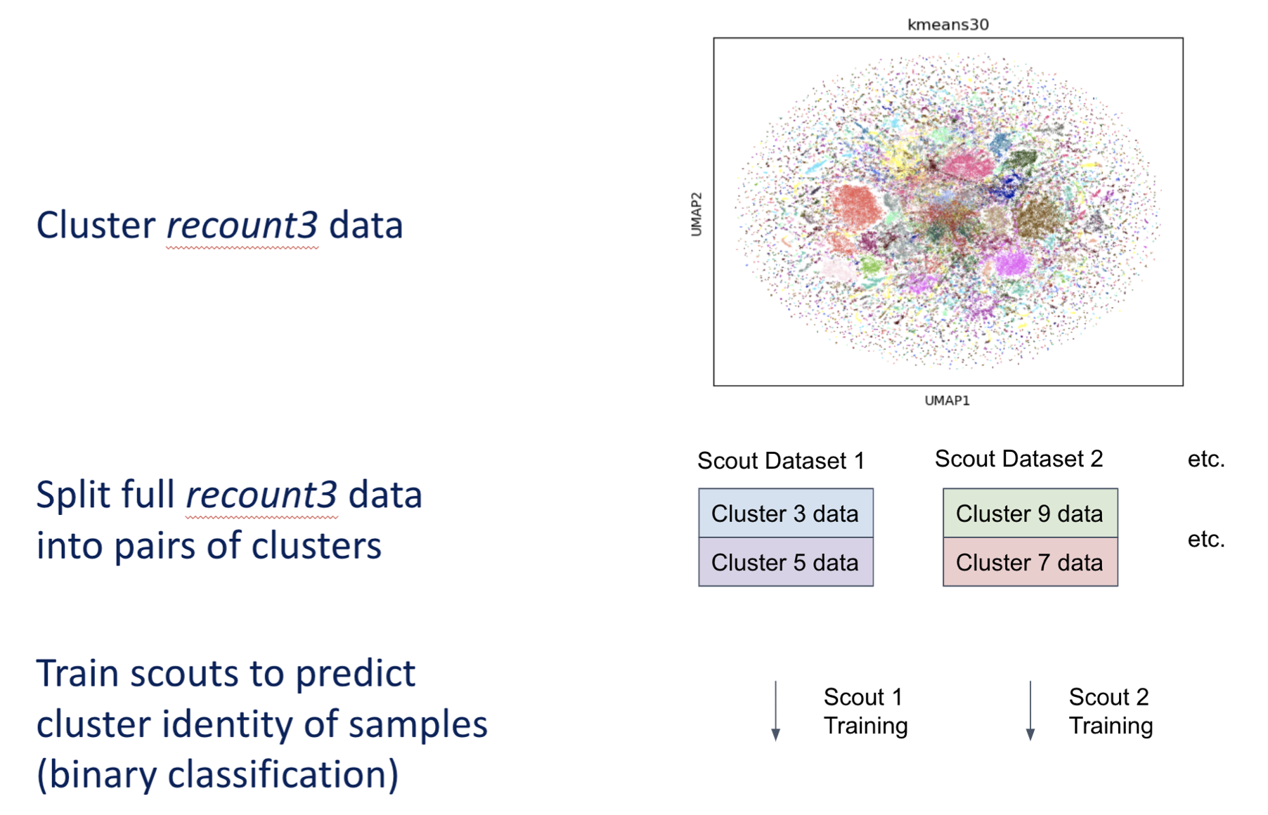
Now, this might seem like a trivial task for the classifier. After all, we are clustering the data based on geometric proximity, then train a model to find decision boundaries between the clusters, so it would seem that the model could find a perfectly clean decision boundary pretty easily. However, keep in mind that the clustering is done in UMAP space, with only the top 30 UMAP components, while the classification is done in the original feature space. UMAP is a nonlinear transformation, so clusters that are easily perfectly separable in top 30 UMAP space may not be in the original space. However, it is definitely still a pretty easy task, but we want the scouting tasks to be doable enough so that the scouts can easily converge to a generalizable relationship. So theoretically, it seems reasonable that this could work! (((Admittedly, it took a lot of playing around before deciding on the above scouting formulation; it just ended up being the one that worked the best. I can’t tell you exactly why, but my reasoning above is the best “intuitve” reasoning I could come up with.)))
GTL pipeline for scBERT: Downstream Task
What about the downstream few-shot task? Here, I will use the same task that I had previously used to evaluate my traditionally pre-trained scBERT model:
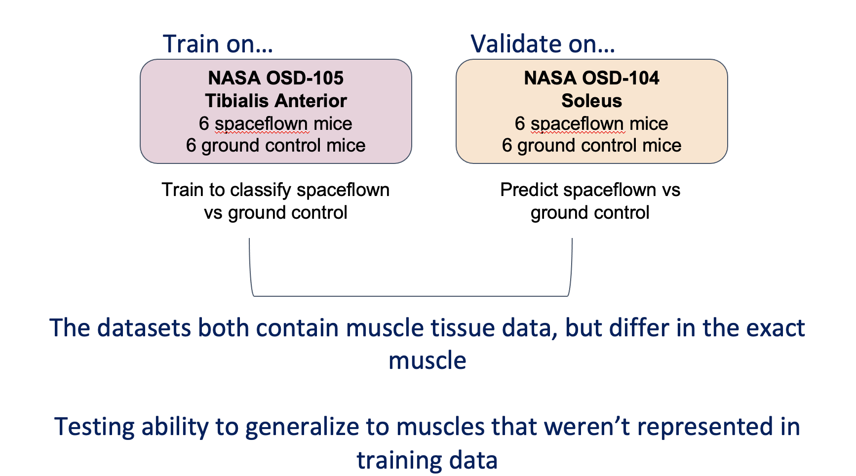
- We train the model on a single NASA OSD dataset, OSD 105
, containing bulk RNA-seq data from 6 spaceflown and 6 ground control mice, and have it predict whether a mouse was spaceflown or ground control. A simple binary classification task, like the scouting problem, but much harder given the incredibly low sample size. - We then validate using another similar NASA OSD dataset, OSD 104
, also containing 6 spaceflown and 6 ground control mice.
It’s important to note that these two datasets, OSD 105 and 104, contain RNA-seq data from different muscle locations. OSD 105 contains tibilalis anterior data, while OSD 104 contains soleus data. However, since these datasets all contain data from some sort of mouse skeletal muscle tissue, we expect that cross-dataset generalizability would be reasonable for a strong generalizable model, and I actually intentionally chose datasets from different muscle tissues to test this difficult problem of cross-tissue generalizability.
GTL pipeline for scBERT: Whole Pipeline
After deciding on the scouting problem formulation, the rest of the pipeline is pretty straightforward. Here’s the full pipeline:
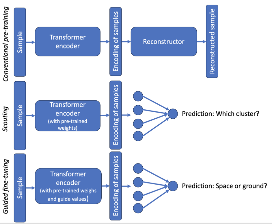
- Pre-train scBERT traditionally on recount3 (self-supervised masked input prediction). This involves the encoder portion of the architecture, which embeds the input, and a reconstructor portion, which uses that embedding to reconstruct the masked input values. The goal here, as always, is to learn general knowledge about the domain (RNA-seq) in the form of good pre-trained weights.
- Scouting on recount3, using the scouting formulation described above. Here, we replace the reconstructor portion of the scBERT architecture with a classification layer. The goal here is, of course, to learn inductive biases in the form of guide values.
- Downstream few-shot fine-tuning on NASA OSDR datasets, using the few-shot formulation described above. Here, we use the same architecture as the scouts. All guide values transfer over!
Results and Analysis
And… here are the results for the downstream task! To compare, I’ve also included results for an scBERT copy that didn’t undergo any pre-training and an scBERT copy that was only traditionally pre-trained on recount3.
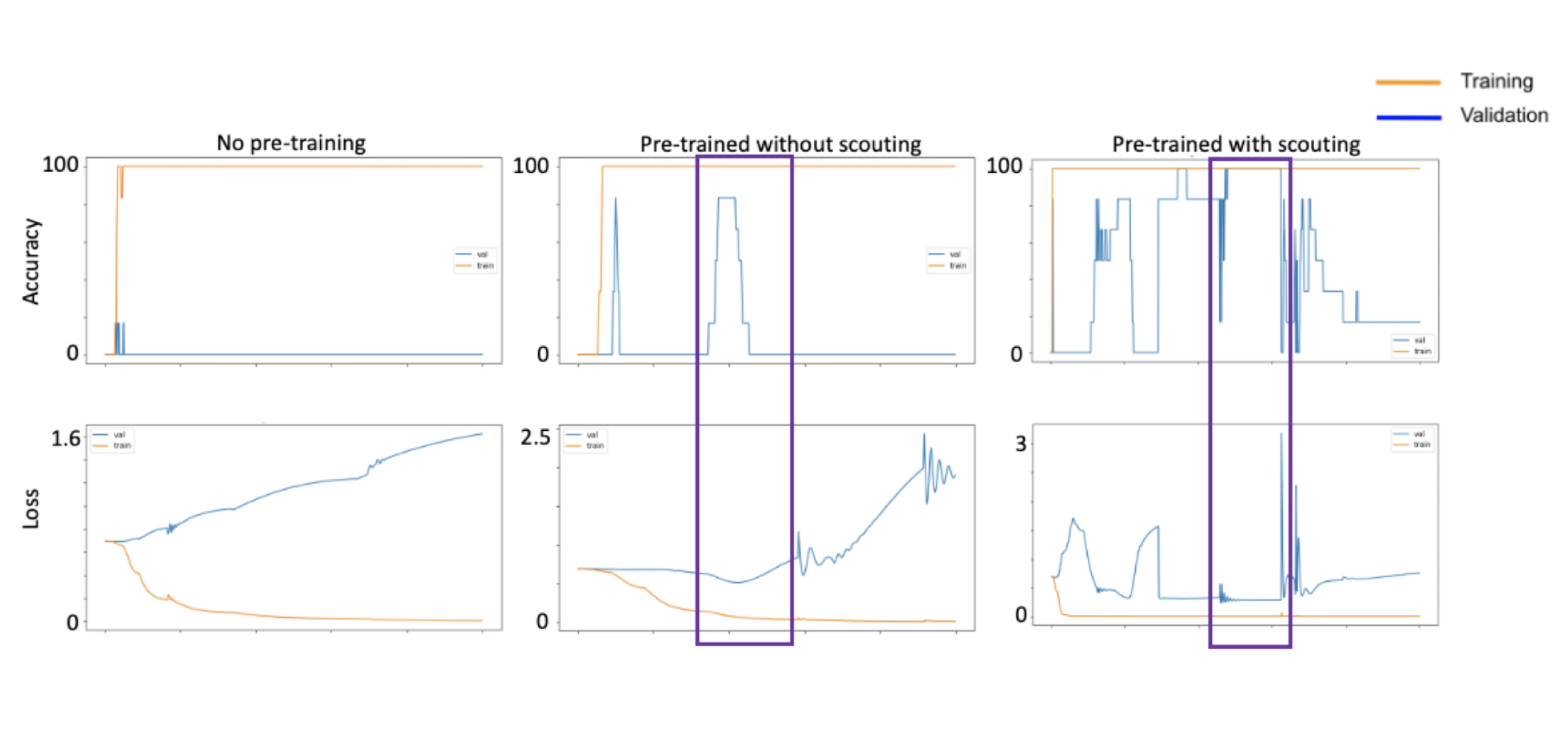
With no pre-training, we can see that severe overfitting to the training set happens almost immediately, with validation loss going up while training loss goes down. This makes sense given the extremely small size of the training set, and the fact that the training and validation sets are from different muscles. With traditional pre-training, however, we see that overfitting also does eventually happen, but right before it happens, at around 200 epochs, we get this sweet spot where validation loss is at a low and validation accuracy is at a high of around 90% (highlighted by the purple box). So it seems that general knowledge about RNA-seq data obtained from traditional pre=training already provides a regularizing effect that reigns in the model from overfitting immediately to the small dowsntream training dataset. These results are from my previous work and are nothing new.
Now, when we add scouting, the max validation accuracy becomes 100%, which is an improvement from the traditionally pre-trained model, though this by itself may not be that notable given the already good validation accuracy after traditional pre-training. What’s potentially more interesting, however, is that this maximum validation performance is maintained over three times as many epochs compared to the traditionally pre-trained model, suggesting that the maximal performance achieved by the GTL model is more robust. However, it is also worth noting that the validation accuracy is a lot noisier and jumps around a lot more for this model compared to the others (keep in mind cosine annealing learning rate scheduler is being used for all these models). But overall, it seems that guided transfer learning provides a more robust regularization effect, giving it a longer period of time with peak validation performance before overfitting occurs.
This is quite exciting, as it shows that, given the right scouting problem setup, we can adapt GTL in settings where our pre-training data is unlabeled, as well! The flexiblity of GTL that allows it to be adapted to such a large variety of scenarios is what, in my eyes, makes this method truly innovative!
Closing Thoughts
Experiment Limitations and Next Steps
These experiements are merely to serve as a preliminary exploration of the nuances of GTL beyond what was presented in the original paper, in hopes that more questions will be explored by the community as GTL gains further publicity and traction. Thus, there is clearly plenty of room for imporvement and next steps regarding these experiments.
For experiement 1, I think it would be cool to establish a more rigorous characterization of the amount of pre-training data (or rather lack thereof) that the addition of GTL can compensate for in terms of downstream performance. This might involve using arious even smaller subsets MNIST and finding the boundary where a pre-training dataset is too small that even GTL cannot compensate for it.
The results of experiment 2 obviously leaves a lot of to be desired, as I only explored single-digit values for the number of categories use in the scout problems. These values are all over an order magnitude off from the number of categories in the downstream task, so none of them gave very useful insight into how “similar” scouting tasks need to be to the downstream task. This was, of course, limited by the MNIST dataset itself, which only had 10 categories. Perhaps using a pre-training dataset with more categories could allow a more comprehensive experiment of this type.
And for experiment 3, I wish I had more time to curate a more robust validation scheme for the downstream few-shot task. A validation set with only 12 samples was really not granular enough to precisely capture the potential benefits of adding GTL on top of traditional transfer learning. When the traditionally pre-trained model is already getting 11/12 prediction correct at its best, is 12/12 really that meaningful of an improvement?
How Exciting is GTL?
As promising as all these results are, GTL is, of course, not the perfect end-all be-all solution to few-shot learning. As was discussed in the original GTL paper and shown in the experiments above, GTL can only provide so much improvement before hitting a wall (e.g. the one-shot learning ability on Omniglot never surpassed 25% validation accuracy). It does not yet quite result in models that match the few-shot learning ability of human intelligence, and still requires a considerable amount of pre-training data. However, the lightweight nature, simplicity, elegance, and adaptibility of the model makes it so that it’s a (relatively) quick and easy solution to get a downstream performance boost on any AI pipelines that already utilize traditional transfer learning!