Training Robust Networks
Exploring ResNet on TinyImageNet, unveiling brittleness and discovering simple robustment enhancement strategies via hyperparameter optimization
Introduction
In the recent years, deep neural networks have emerged as a dominant force in the field of machine learning, achieving remarkable success across a variety of tasks, from VGG-16 in image classification to ChatGPT in natural language modeling. However, the very complexity that allows deep neural networks to learn and represent complex patterns and relationships can also leave them susceptible to challenges such as overfitting, adversarial attacks, and interpretability. The brittleness of deep neural networks, in particular, poses a significant challenge toward their deployment in real-world applications, especially those where reliability is paramount, like medical image diagnosis and autonomous vehicle navigation. Consequently, it is crucial to develop a better understanding of deep architectures and explore strategies for enhancing robustness. This project focuses specifically on ResNet, a model introduced in 2015 for image classification that is still widely used today. In particular, we study the model’s vulnerability to adversarial perturbations and, subsequently, work through a strategy to enhance its resilience through data augmentation and hyperparameter optimization.
Related Works
ResNet


The brittleness of many deep neural networks for computer vision, including ResNet, is well documented. For example, adding a tiny amount of random Gaussian noise, imperceptible to the human eye, can dramatically affect the accuracy and confidence of a network. In fact, we can optimize over the input image to generate small, non-random perturbations that can be used to alter the network’s prediction behavior arbitrarily, a vulnerability that applies to a variety of networks
In this project, we investigate two small perturbations: adding random Gaussian noise and modifying the colors of a small subset of pixels. We use hyperparameter search to fine-tune ResNet-18, aiming to create a network robust to these perturbations without compromising significantly on accuracy. Specifically, we examine general hyperparameters like batch size, learning rate, number of frozen layers, and more. The ultimate goal is to define a straightforward and resource-efficient strategy for mitigating brittleness that can potentially be extended to other architectures and domains.
Methodology
Baseline Model
The out-of-the-box ResNet18 model is pretrained on ImageNet, achieving about 55% accuracy on the ImageNet validation set. TinyImageNet is a subset of ImageNet with fewer classes; there is a potential need for further fine-tuning of the out-of-the-box model to optimize performance. Thus, we start off by performing a simple hyperparameter grid search over batch size and learning rate. Each model is trained on the TinyImageNet training set, a dataset of 40,000 images (downsampled from 100,000 for computational ease) with 200 classes (roughly uniform class distribution). The baseline model is then selected based on accuracy on the TinyImageNet validation set, a uniformly balanced dataset of 10,000 images.
Generating Adversarial Perturbations
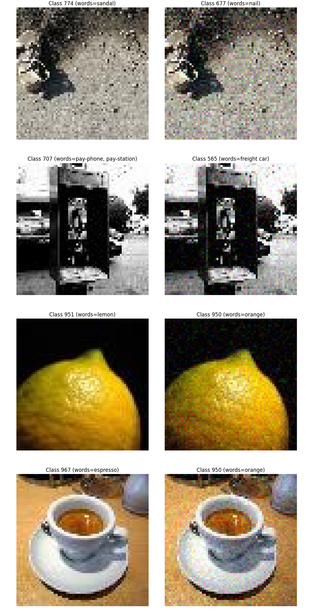
Next, we use gradient descent to create adversarial perturbations. The first perturbation is adding a small amount of Gaussian noise. We try to maximize the probability of the input image belonging to a wrong class (the inverse of the standard cross-entropy classification objective) while also penalizing the magnitude of the noise. This approach is more efficient and controllable compared to attempting to add a random sample of Gaussian noise with the hope of inducing misclassification.

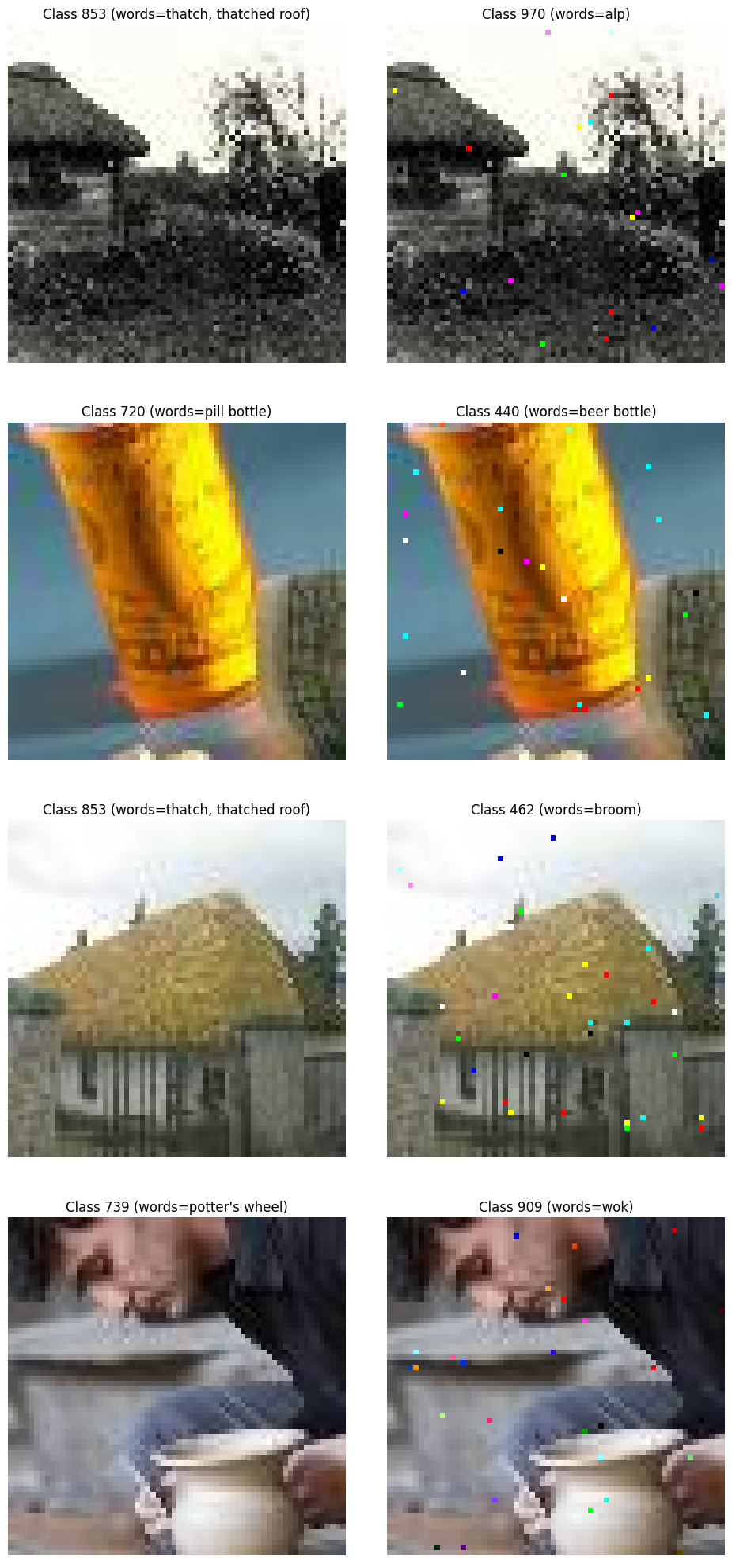
The other perturbation is randomly selecting a small subset of pixels (0.5%) and adjusting their color until the image is misclassified by the baseline model. A gradient descent approach that maximizes the probability of the input image belong to a wrong class is used to implement this perturbation; however, it is much more sensitive to initialization and can require retries, making it less resource-efficient.

We generate 11,000 adversarial examples using the Gaussian noise perturbation technique on the training examples that the baseline model correctly classifies. Of these adversarial examples, we use 10,000 of them to augment the training dataset (call it the augmented training set) and reserve 1,000 for hyperparameter optimization (call it the perturbed training set). We also generate 2,000 adversarial examples using the same perturbation technique on the validation examples that the baseline model correctly classifies. 1,000 of these are used for hyperparameter optimization (call it the perturbed validation set) while the rest are saved for out-of-sample evaluation (call it the hold-out validation set).
Note that we keep adversarial examples generated from the validation set out of the augmented training set to avoid lookahead bias. We want to avoid allowing the model to gain insights into the characteristics of examples that it will encounter in the validation set (since perturbed images are very similar to the original images), ensuring a more accurate assessment of the model’s robustness and generalization capabilities.
Finally, we generate an additional 500 examples using the pixel modification perturbation technique on the validation examples that the baseline correctly classifies (call it the out-of-distribution hold-out set). These examples are reserved for out-of-sample and out-of-distribution evaluation, assessing the model’s ability to perform well on adversarial perturbations it has never seen before.
Hyperparameter Optimization to Create a More Robust Model
Equipped with the augmented/additional datasets from the previous step, we start the process of model creation. The relevant metrics for selecting a model are original validation accuracy (derived from the original validation dataset from TinyImageNet), perturbed training accuracy, and perturbed validation accuracy. It is crucial to look at original validation accuracy to ensure that we are not creating robust models by compromising significantly on the original image classification task. In addition, accuracy on the perturbed train dataset tells us how well our model adjusts to the perturbation, while accuracy on the perturbed validation dataset provides an additional perspective by evaluating how well the model generalizes to perturbations on images it has never seen before. The same set of metrics is used in evaluating the final model on out-of-sample datasets, in addition to accuracy on the out-of-distribution hold-out set.
We examine how varying four different hyperparameters affects the robustness of ResNet-18. The first hyperparameter involves initializing the model with either weights from the baseline model or the default pre-trained weights. The next hyperparameter is how many layers of ResNet-18 are frozen during the training procedure. The last two hyperparameters are batch size and learning rate. It is important to note that we do not conduct a search over a four-dimensional hyperparameter grid for computational reasons. Instead, we fix some hyperparameters at reasonable default values while we vary over the other hyperparameters. Using the insights gleaned from this hyperparameter search, we proceed to train the final model.
Comparing Models via Visualization
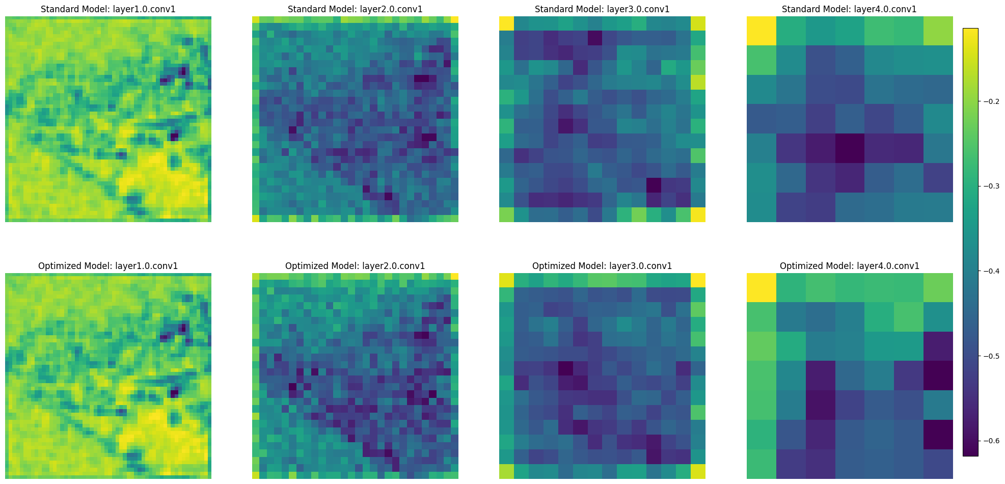
Finally, we transform the feature maps generated for an input image into interpretable visualizations to better understand the learned representations within the models. These feature maps capture the activations of learned filters or kernels across different regions of the input images and are the basis for our analysis
Layer: conv1, Activation shape: torch.Size([1, 64, 112, 112])
Layer: layer1.0.conv1, Activation shape: torch.Size([1, 64, 56, 56])
Layer: layer1.0.conv2, Activation shape: torch.Size([1, 64, 56, 56])
Layer: layer1.1.conv1, Activation shape: torch.Size([1, 64, 56, 56])
Layer: layer1.1.conv2, Activation shape: torch.Size([1, 64, 56, 56])
Layer: layer2.0.conv1, Activation shape: torch.Size([1, 128, 28, 28])
Layer: layer2.0.conv2, Activation shape: torch.Size([1, 128, 28, 28])
Layer: layer2.0.downsample.0, Activation shape: torch.Size([1, 128, 28, 28])
Layer: layer2.1.conv1, Activation shape: torch.Size([1, 128, 28, 28])
Layer: layer2.1.conv2, Activation shape: torch.Size([1, 128, 28, 28])
Layer: layer3.0.conv1, Activation shape: torch.Size([1, 256, 14, 14])
Layer: layer3.0.conv2, Activation shape: torch.Size([1, 256, 14, 14])
Layer: layer3.0.downsample.0, Activation shape: torch.Size([1, 256, 14, 14])
Layer: layer3.1.conv1, Activation shape: torch.Size([1, 256, 14, 14])
Layer: layer3.1.conv2, Activation shape: torch.Size([1, 256, 14, 14])
Layer: layer4.0.conv1, Activation shape: torch.Size([1, 512, 7, 7])
Layer: layer4.0.conv2, Activation shape: torch.Size([1, 512, 7, 7])
Layer: layer4.0.downsample.0, Activation shape: torch.Size([1, 512, 7, 7])
Layer: layer4.1.conv1, Activation shape: torch.Size([1, 512, 7, 7])
Layer: layer4.1.conv2, Activation shape: torch.Size([1, 512, 7, 7])
Layer: fc, Activation shape: torch.Size([1, 1000])
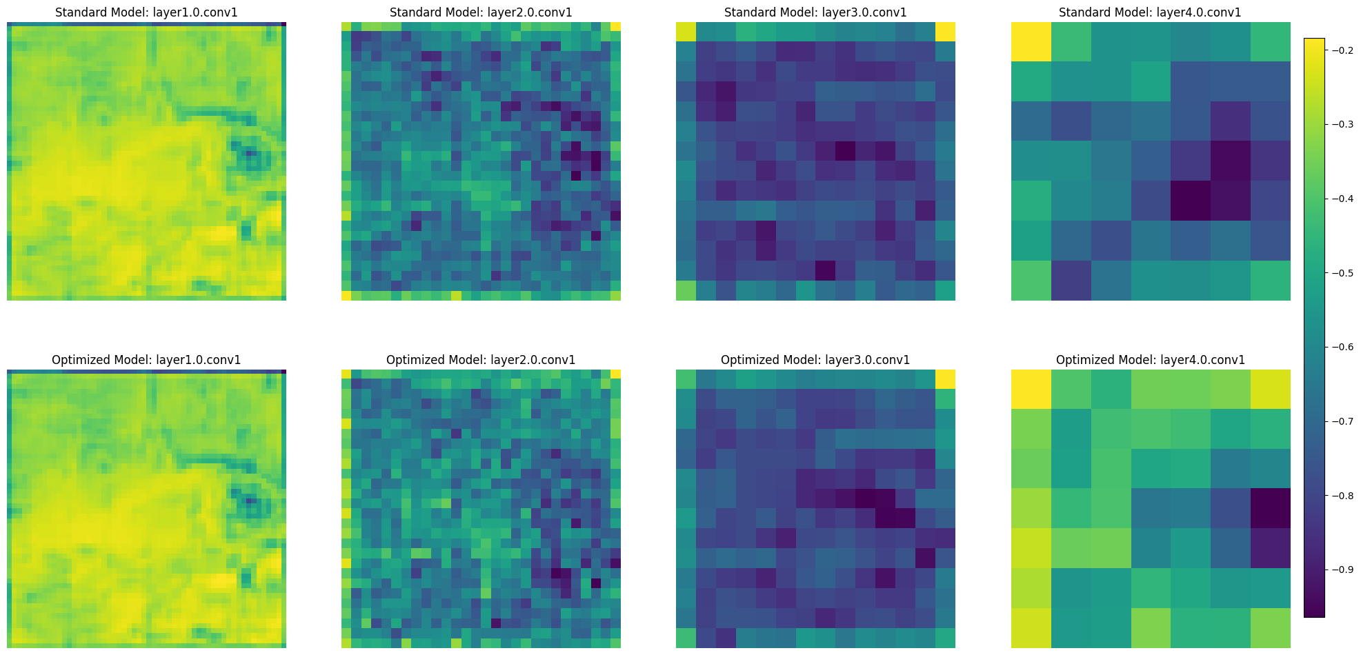
After obtaining these activations, we compute the average activation values across the channels (neurons) within a specified layer of interest. This process provides insights into which regions or patterns in the input images contribute significantly to the neuron activations within that layer. We then create heatmap visualizations based on these average activations, highlighting the areas of the input data that have the most substantial impact on the network’s feature detection process. This allows us to gain valuable insights into how the network perceives and prioritizes various features across its layers, aiding in our understanding of the model’s inner workings.
We use this approach to compare the baseline model to the final model, aiming to identify significant differences in feature prioritization or the patterns detected at various layers.
Results and Discussion
Baseline Model
First, we perform a grid search over batch sizes ranging from 128 to 512 and learning rates ranging from 0.0001 to 0.01.
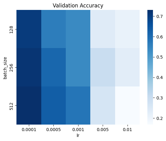
The results from the first hyperparameter search suggest that conservative learning rates and large batch sizes lead to good performance. Thus, we perform a finer grid search over batch sizes ranging from 256 to 512 and learning rates ranging from 0.00001 to 0.0001.
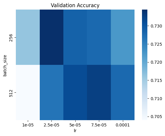
Based on the results from the second hyperparameter search, we choose our baseline model to be ResNet-18 fine-tuned with a batch size of 256 and a learning rate of 0.00005. The baseline model achieves nearly 73% accuracy on the validation set, which is possibly due to the fact that TinyImageNet has less classes, so classification may be an easier task.
Effect of Hyperparameters
Number of Unfrozen Layers
Next, we evaluate how the number of unfrozen layers (up to 3) affects the robustness of the trained models, whose weights can either be initialized from the baseline model or from the pre-trained/default model (in the diagram below, is_finetuned=True corresponds to the baseline model).
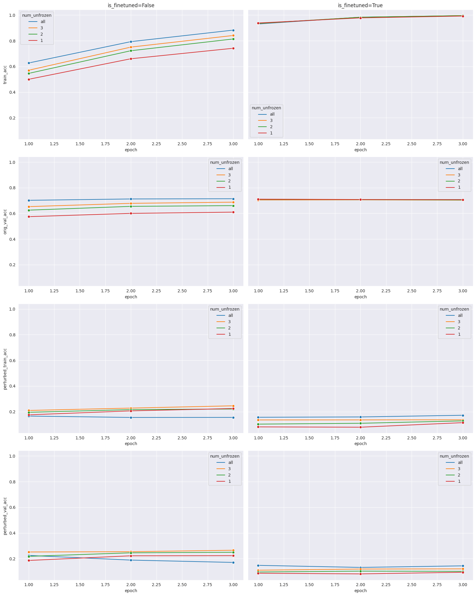
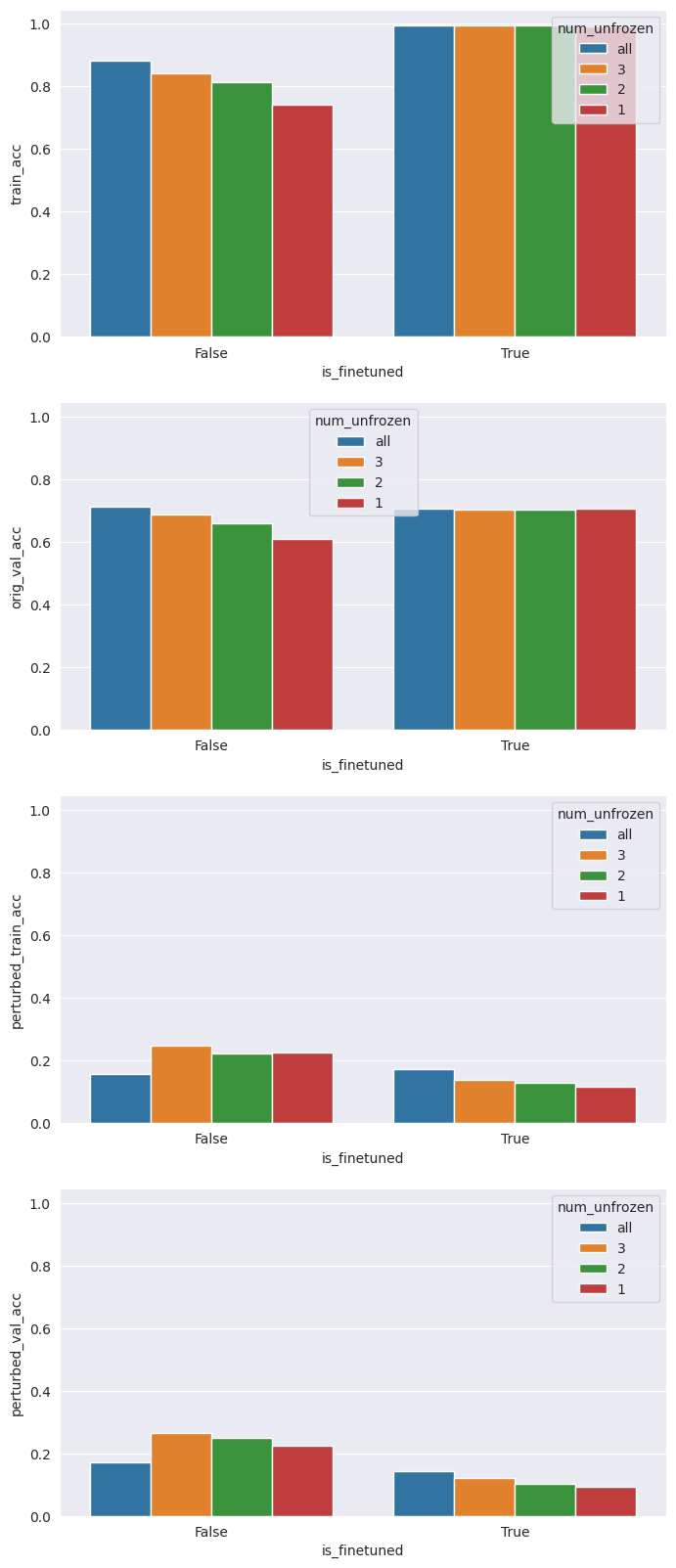
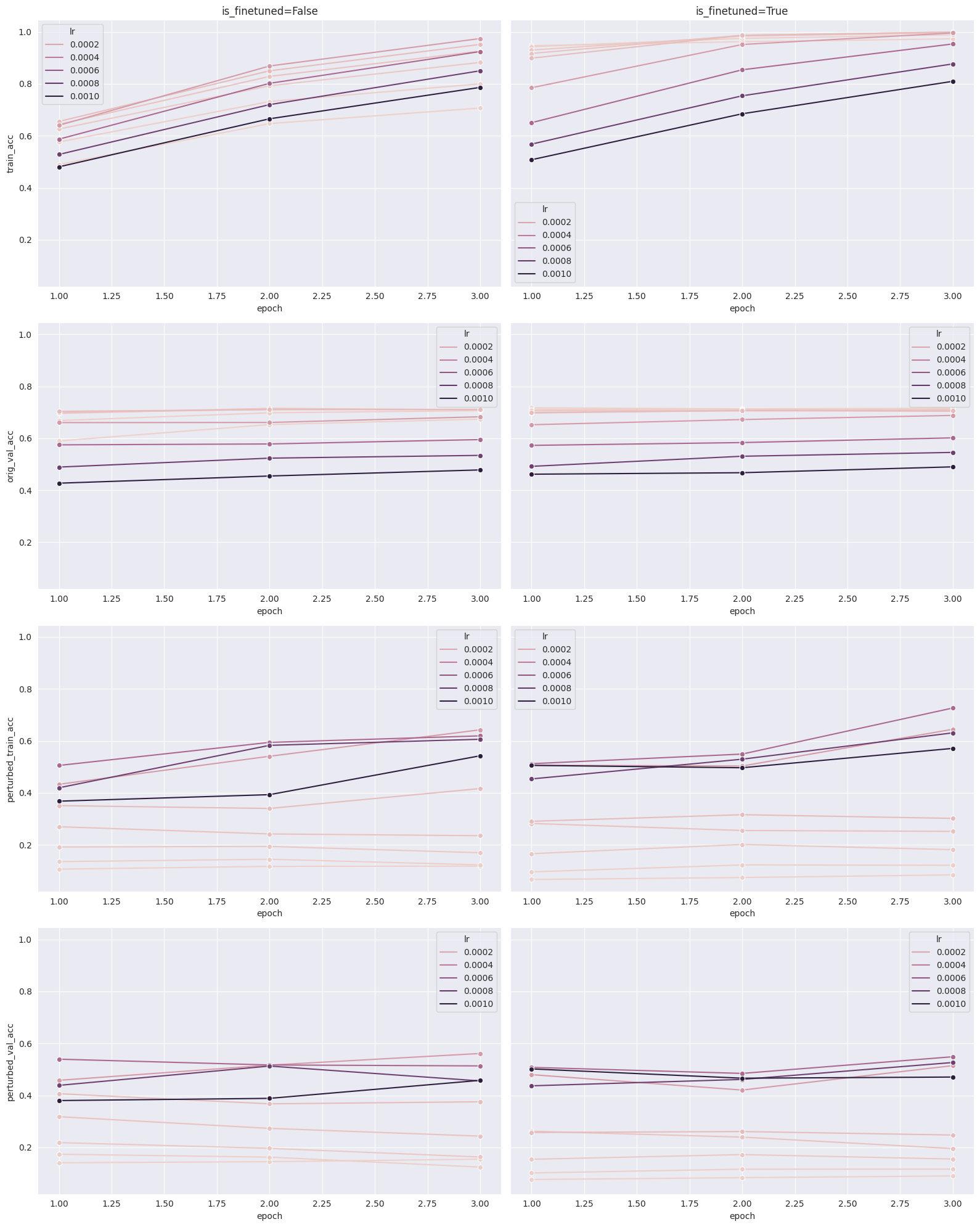
First, we observe that training for more epochs does not improve the metrics of interest. This implies that training for robustness can be computationally efficient. Next, we observe there is a substantial drop in accuracy for the perturbed datasets compared to the original validation dataset, which is to be expected. Pairing the accuracies for the perturbed datasets across hyperparameter combinations, we observe that they are tightly correlated, which implies that our models are effectively adapting to the perturbation.
One interesting observation to note here is that accuracies on the perturbed datasets are significantly higher for the model initialized with default weights (27% compared to 10%). An intuitive explanation for this is that we have deliberately engineered a brittle baseline model, so the model is in a region of the optimization landscape characterized by high accuracy but low robustness. If we want achieve high accuracy and high robustness, we may need to start from a less unfavorable position in the optimization landscape.
Finally, we observe that freezing some layers can enhance robustness for models initialized from the default weights at the cost of performance on the original task. This aligns with intuition, since allowing all the weights to vary can lead to overfitting, resulting in more brittle networks.
Batch Size
Next, we evaluate how batch size (ranging from 4 to 512) affects the robustness of the trained models.
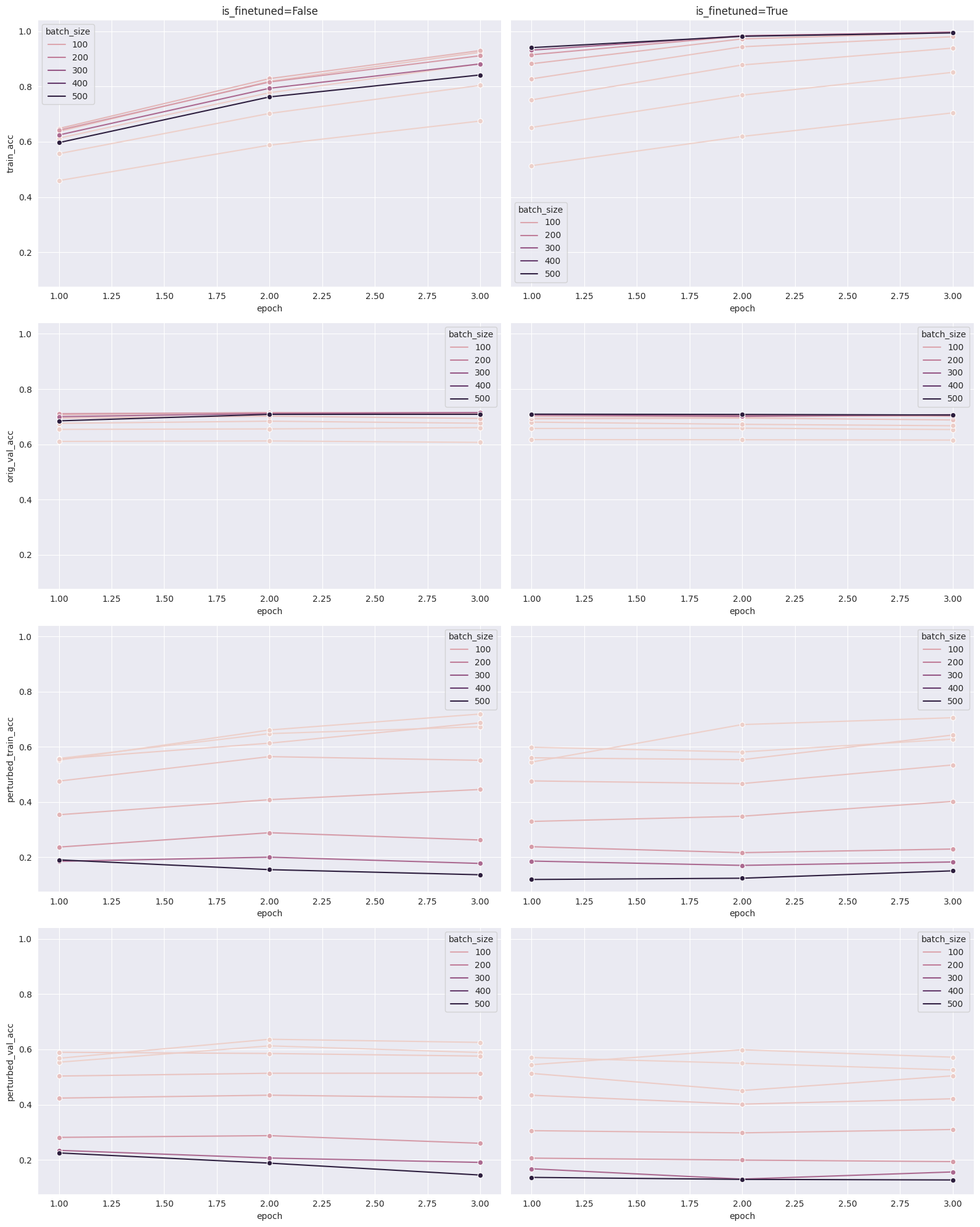
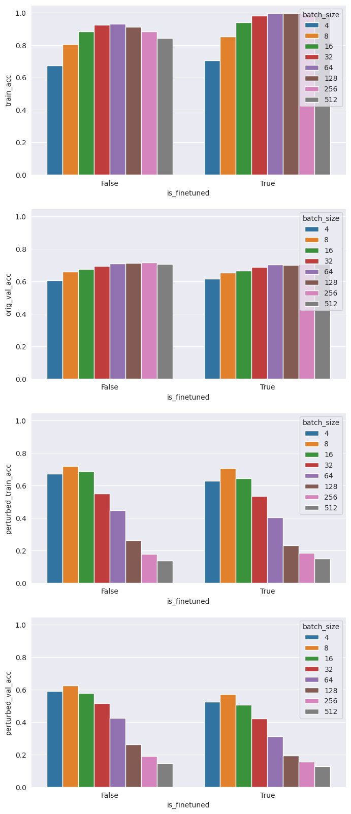
We notice immediately that batch size has a considerable effect on robustness. For both the perturbed training set and the perturbed validation set, accuracies are markedly lower with large batch sizes (around 15%) and higher with small batch sizes (around 70%). As expected, this comes at the expense of lower performance on the original task, with original validation accuracy dropping 10% as the batch size decreases from 512 to 4. Depending on the use case, this may be an efficient tradeoff to make!
Learning Rate
Finally, we evaluate how learning rate (ranging from 0.00001 to 0.001) affects the robustness of the trained models.
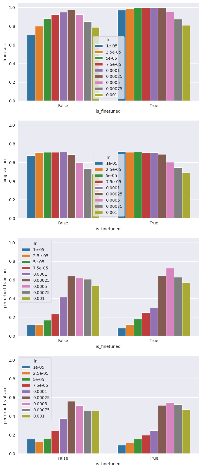
Like batch size, learning rate significantly impacts robustness. The sweet spot for learning rate in terms of robustness seems to be around 0.00025, with original validation accuracy dropping as the learning rate becomes more conservative; a learning rate of 0.00025 leads to a 3% drop in performance. Like before, this may be a worthwhile tradeoff to make.
Out of Sample Evaluation
Using the insights gained from the hyperparameter search, we define the final model with the following hyperparameters:
is_finetuned=False
num_unfrozen_layers=3
batch_size=8
learning_rate=0.00025
Of course, this is likely not the optimal hyperparameter combination, since we were not able to perform a full grid search. The results are as follows:
| Dataset | Accuracy |
|---|---|
| Original validation | 0.522754 |
| Perturbed training | 0.569572 |
| Perturbed validation | 0.442720 |
| Hold-out validation | 0.485621 |
| Out-of-distribution validation | 0.489786 |
Original validation, perturbed validation, and hold-out validation accuracy are somewhat lower than the optimistic estimates derived from the hyperparameter search. However, we observe that we are able to achieve nearly 50% accuracy on the out-of-distribution validation set, which contains pixel modification perturbations that the model was never trained on, underscoring the robustness and adaptability of our model.
Model Comparison
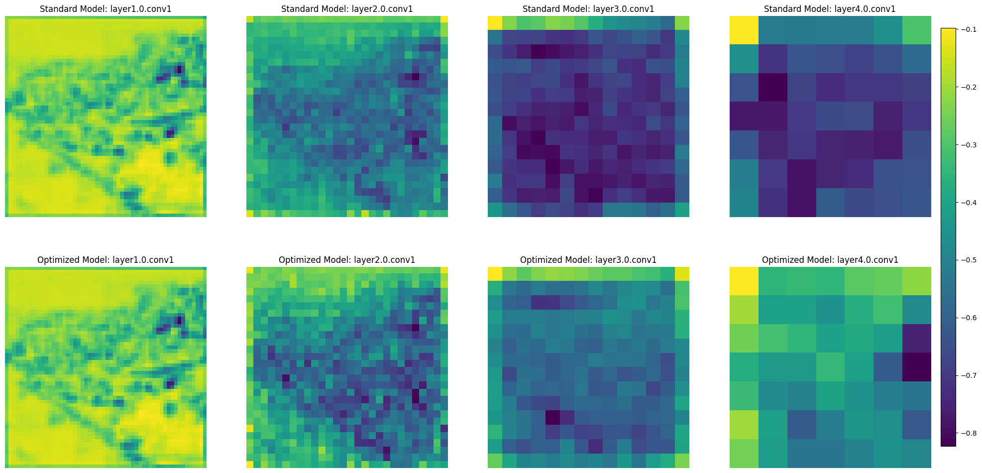
Lastly, we observe the progression of feature map representations: starting from basic visual elements such as edges and textures in the initial layers, to more complex patterns in intermediate layers, and culminating in sophisticated, high-level feature representations in the deeper layers. This layered evolution is integral to the network’s ability to analyze and recognize complex images.
When comparing the baseline model to the final model, there are very few (if any) differences in the initial layers. By the intermediate and deeper layers, there are clear differences in which aspects of the images have the greatest activation. This observation aligns with the foundational principles of convolutional neural networks, where initial layers tend to be more generic, capturing universal features that are commonly useful across various tasks. As a result, the similarity in the initial layers between the baseline and final models suggests that these early representations are robust and essential for basic image processing, irrespective of specific model optimizations or task-focused training.
However, the divergence observed in the intermediate and deeper layers is indicative of the specialized learning that occurs as a result of hyperparameter tuning in the final model. These layers, being more task-specific, have adapted to capture more complex and abstract features relevant to the particular objectives of the final model.
Conclusion and Next Steps
In this project, we have undertaken a comprehensive exploration of enhancing ResNet through data augmentation with adversarial examples and straightforward hyperparameter tuning. Key highlights include the computational efficiency and simplicity of the employed technique, the resulting model’s ability to adapt to both seen and unseen perturbations, and the capacity to finely control tradeoffs between robustness and accuracy thorugh the manipulation of diverse hyperparameters.
There are many potential avenues for future exploration. One prospect involves expanding and refining the discussed techniques by continuing to explore the hyperparameter space, considering additional parameters or refining the search range. Additionally, applying this analysis to different architectures and domains could reveal further insights. Finally, broadening the scope of perturbations presents another avenue, offering the potential to develop more practical models tailored for real-world applications.