Autoen-chorder: Predicting Musical Success With Neural Nets
In this blog, we discuss deep learning methods and results of predicting song popularity from audio features.
Introduction
Our aim is to use deep learning (the crux of 6.s898) to help musicians and their sponsors (for example: agents, record labels, and investors) identify whether songs will resonate with listeners. Solving this problem would enable established artists to release more impactful music, and spur new musicians to break into a competitive market.
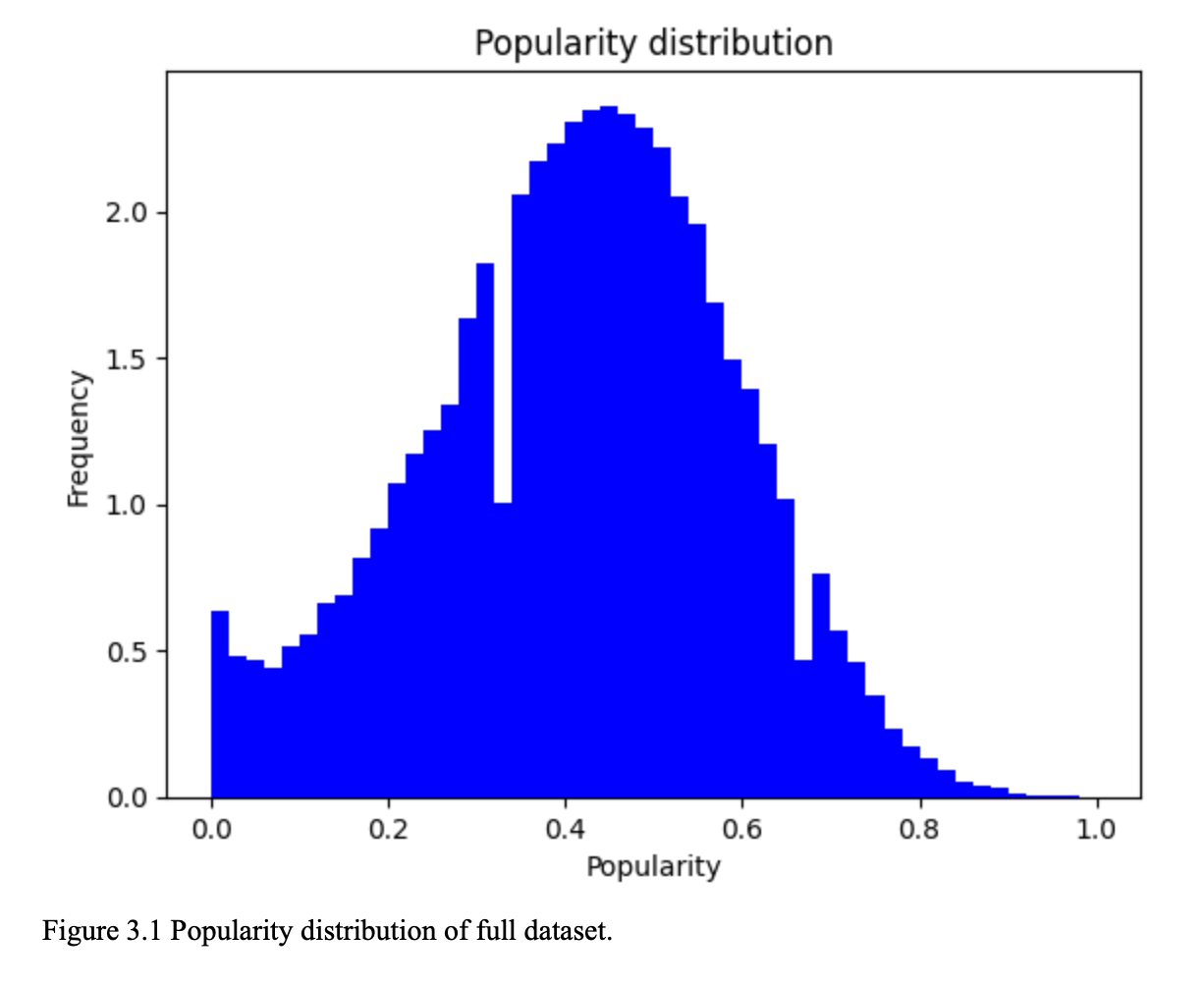
We first begin by establishing what our success metric is. For the purposes of this project, we will use the concept of song “popularity” as the metric we want to predict, and we source our popularity data from the SpotGenTrack Popularity Dataset. This dataset leverages Spotify’s Popularity Index, which is a relative rank measured against other songs’ popularities. It is a function of recent stream count, save rate, playlist appearance count, skip rate, share rate, and more.
There already exist a few models to help us solve this problem. However, these models make use of metadata, such as artist name, year of release, and genre. We believe that these models – while interesting – are insufficient to be actionable, particularly for up-and-coming musicians who may be innovating new music genres, or who may not yet have a strong name. Specifically, metadata like Artist Name are both highly-weighted (for example, even Taylor Swift’s least popular song will be a relative superhit) and unchangeable (we cannot suggest that artists change their identity to Beyonce). Additionally, features like Genre are imprecise, and can quickly become outdated as new subgenres and crossover genres are developed.
To address this gap and become more actionable to musicians, we aimed to create a new model that can achieve near-parity with metadata-based models without leveraging any metadata. By combining multiple audio-feature models, we not only achieved comparable results to metadata-based models, we actually outperformed metadata-based models on more than half our testing data.
Previous Works
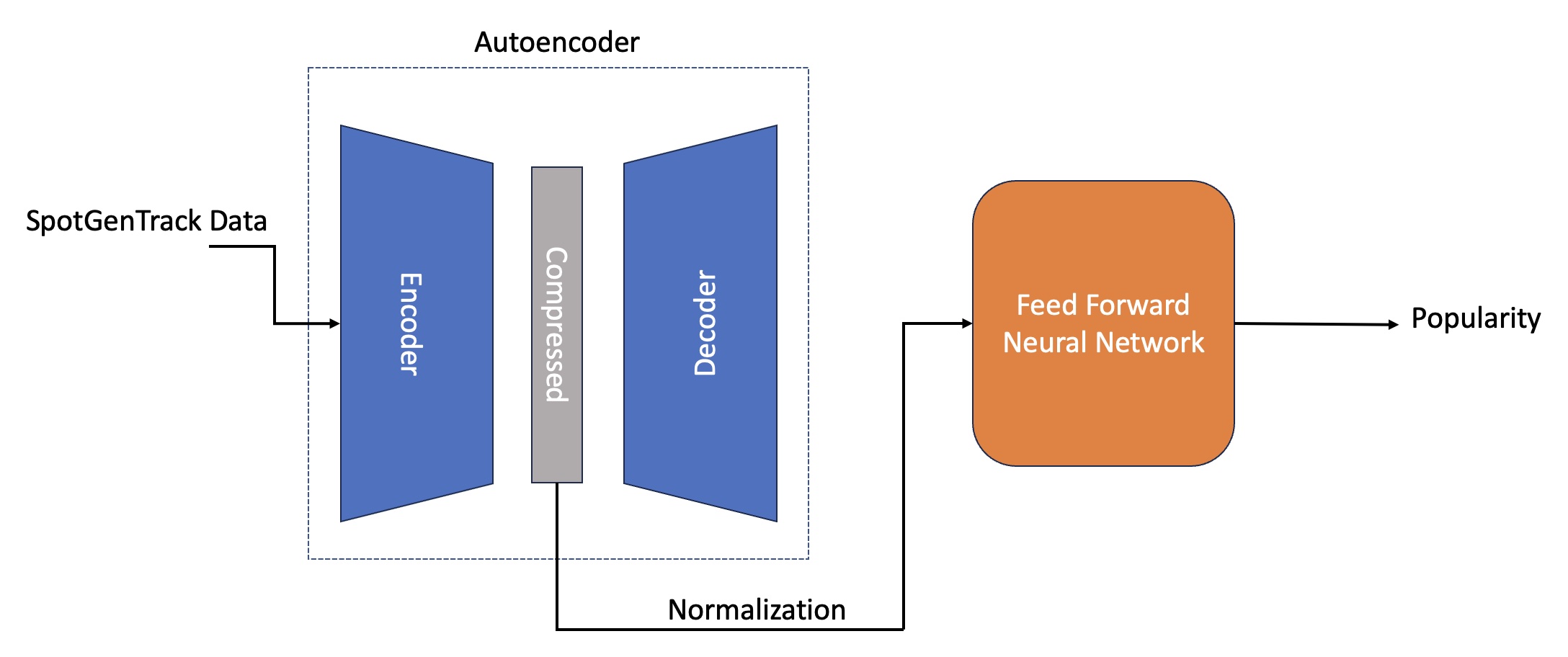
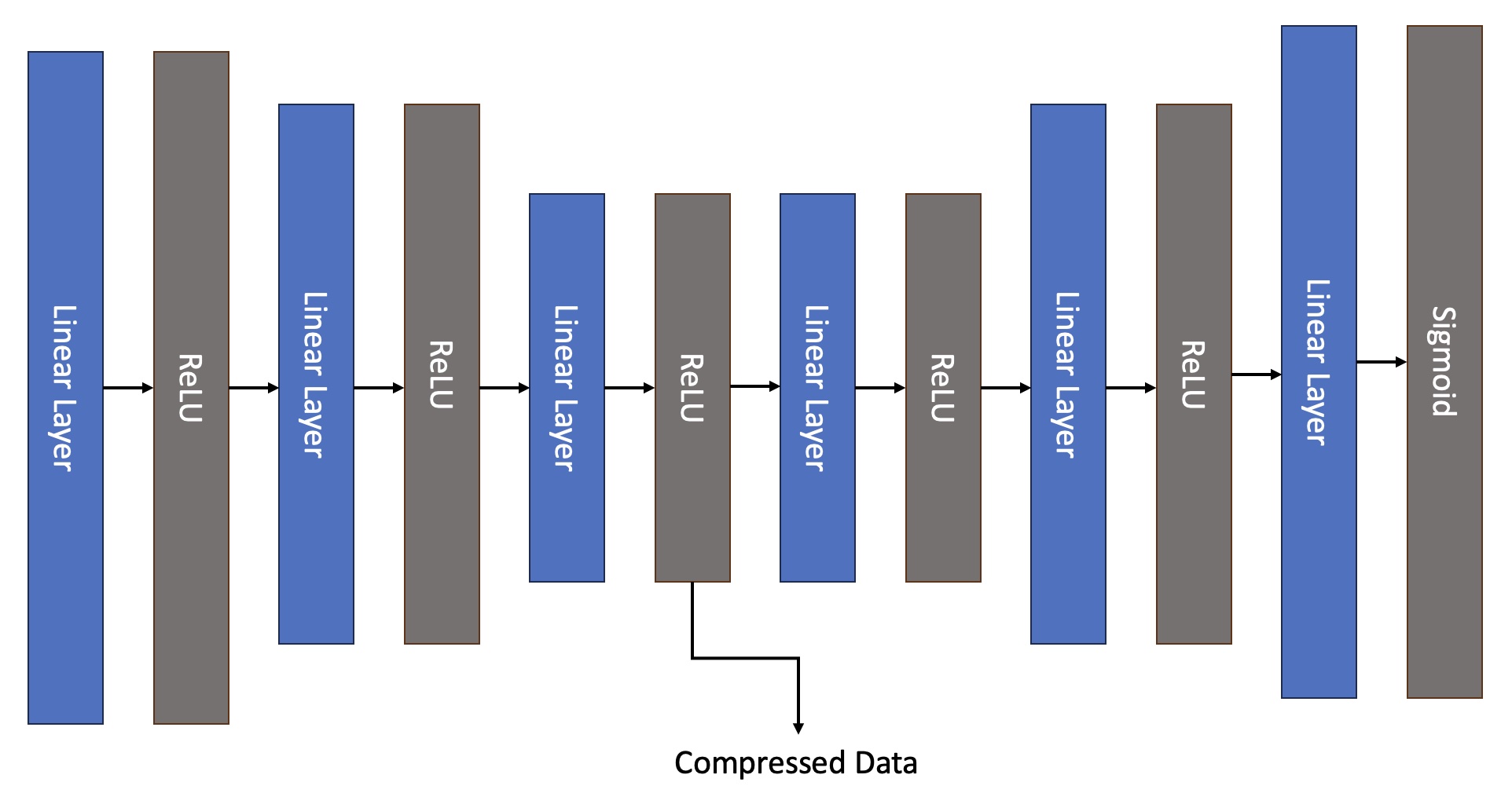
The most prominent existing model is HitMusicNet (heretofore referred to as “HMN”). The HMN model predicts popularity based on lyric data from Genius.com (syllables, words, etc.), high-level audio features from SpotGenTrack (e.g. acousticness, key, tempo, speechiness), low-level audio features from SpotGenTrack (audio preprocessing, such as spectral analyses), and metadata from SpotGenTrack (e.g. artist name, year of release, genre). A feature vector is created with this information, and said vector is fed as the input into an Autoencoder network to compress the features, followed by a neural network to obtain the predicted popularity.
HitMusicNet has two different objectives: Regression and classification. For this project, we will focus only on regression since it will allow us to visualize differences between our model and HMN with higher granularity. We replicated the code from the paper in PyTorch, using the same functions and data and calculated metrics to make sure our implementation is correctly replicating the paper. We see a slight discrepancy in the errors, likely due to the test/train split during the paper’s training. Altogether, we can still consider our replicated model as valid as the metrics are within reasonable range to the reported metrics. Additionally, we added the R-squared metric as an additional metric to ensure our model fits the data.

A second model, VGGish, is a pretrained convolutional neural network trained on YouTube-100M (a database with 100 million YouTube videos). This network is a representation learning network widely used in established papers. This network takes in a wav file and processes it on 0.96-second windows, and calculates 128 embeddings per window. This means that the resulting tensor from VGGish will be 2 dimensional for a single file, and 3 dimensional for a batch of files.
Hypothesis
HMN has a tendency to be heavily-indexed on metadata features and lyrics. Data such as artist name heavily bias the model’s popularity predictions in favor of big-name artists. Lyrics information can make the model biased to predicting instrumental music as less likely to be successful. While this may be representative of how the industry works, it makes HMN much less actionable for musicians trying to assess their chance of success with the market.
We believe that audio-only features – such as temporal information (i.e. the structure of the song and information about previous sections) and repetition – can alone be fairly successful in determining a song’s popularity. Thus, we chose to use just audio data, as well as temporal data, to predict popularity.
We hypothesize that combining the audio-only features of HMN with VGGish’s audio representation will yield superior outcomes to HMN’s audio-only features alone. We also hope that our new model can compete with the full HMN model (i.e. audio features and metadata combined).
Data Preprocessing
Given our hypothesis, we need to extract the low-level features from our signal and map each row to its corresponding audio file to be fed into VGGish. We used Spotify’s API to obtain the raw audio files to be processed, and then ran them through the VGGish network. We performed the same preprocessing as the one done in the MusicHitNet paper.
File length limitation
Unfourtunately, Spotify only allows the download of 30s previews of songs.
Memory limitation
Audio files are heavy, and the longer they are, the heavier. We should ideally process all 95,000 songs’ full length, but given Spotify’s API’s request limit, and the size of the files, we were only able to obtain 10,000 30s snippets. This still resulted in roughly 14.5 GB of data. Processing the whole dataset would not only require roughly 140 GBs of data, but the Spotify API’s limits will likely be exceeded, and our colab notebook will likely run out of memory.
Downsampling and splitting
Given the considerations above, we decided to use 10,000 songs for our model’s development, splitting the data into 8,500 samples for training and 1,500 for validation. Given that this is roughly 10% of the original data, we expect the model’s performance to be below the reported metrics.
Baselines
The metrics obtained when replicating the HMN network serve as a reasonable parameter to verify our model’s accuracy. As mentioned above, the model’s performance is expected to be below the paper’s reported metrics. To understand the range, we retrained a network with the same shape as the paper’s using the 10,000 samples in the same train/test split we will feed to our new network. The resulting metrics for this experiment can be seen in Table 2.

Training a model that results in similar metrics would be ideal, but realistically, as we will only be using low-level data, we expect the metrics to be lower than the values in Table 2. To ensure that our trained model isn’t just predicting noise, we use a baseline comparison, comparing against a random normal distribution with mean μ=40.02 and σ=16.79.

As seen in table 3, the baseline intuitively would not appear to be too far from the trained HMN model in terms of MSE and MAE. When looking at the r-squared, the random model has a negative value, while the trained HMN netw ork results with a much higher 0.5616 value. To deem a model as successful, we will compare it against both sets of metrics.
Alternate Models
- Single autoencoder. Our first iteration to solve this problem consisted of using a single autoencoder to find representations with data coming from VGGish and SpotGetTrack low level features, and then running that through a feed-forward network similar to the one used in HMN. Since the output of VGGish is a tensor of shape (batch_size, n_windows, n_features) and the output of SpotGenTrack is (batch_size, 207), we concluded there was no simple way to combine the two data sources without losing temporal information.
- RNN. Our second iteration consisted of running the data coming from SpotGenTrack Low-Level through an autoencoder in the same way HMN does it. After this initial train gives us a compressed representation of the data from SpotGenTrack Low-Level, we train two subsequent networks: First an LSTM RNN which transforms data into (batch_size, 20), then we add the compressed representation from SpotGenTrack Low-Level and run that through a feedforward network. This model yielded a performance below the baseline.
- HMN+VGGish: This model consists of taking the full SpotGenTrack data, passing it through the regular autoencoder defined in HMN, and add it to the output coming from VGGish. This model, while resulting in promising results, still yielded worse performance than HMN on its own, so our team decided to explore alternatives.
- LossNet. Our third exploration consisted of training a model that uses VGGish’s outputs to try and predict losses from HMN. In essence, we are trying to use VGGish Representation to capture information that HMN consistently is unable to. This approach has parallels with Adversarial Networks, in that one model is being trained on the losses of another model. However, this approach is more cooperative than adversarial, since the result of the two models is not zero-sum. This approach led to a dead-end with surprising results.
Final Architecture
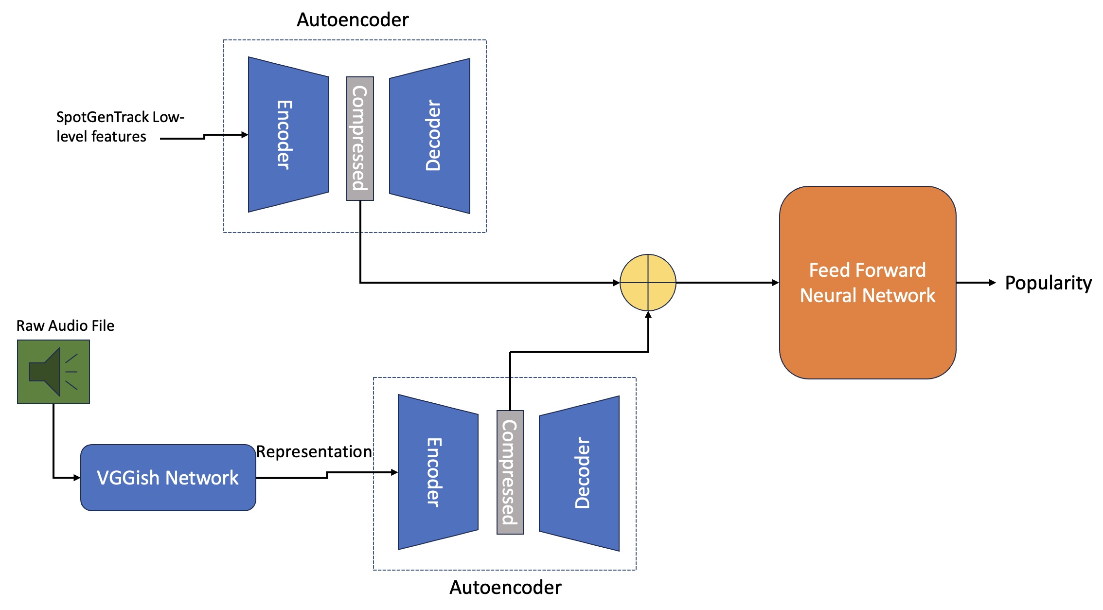
Our final iteration consists of a model with two autoencoders: One for data from SpotGenTrack low level features, the second for the representation obtained using the VGGish model. The slight difference between these two models is that the VGGish autoencoder has additional LSTM layers at the start of the encoder, and at the end of the decoder. The output from these two autoencoders is then added together and passed through a feed-forward network. This architecture can be seen in Figure 4.
Padding and Packing
None of the audio files coming from Spotify previews are more than 30s in duration, but some are in fact shorter than others. To solve this issue, and also to be able to feed our model whichever sized data we require, we use pytorch’s packing functionality. Packing allows us to process sequential data with different sizes, so that only the relevant information is passed through the LSTM. Conversely, padding allows us to add zeros at the end of sequences so that all samples have the same size. This is required to store data in tensors.
Hyperparameters
Additional Model Considerations
The original HMN model compiles 228 features into 45 representations for the feed-forward network. We want our model’s feed-forward network to have a similar number of inputs as the given architecture, therefore we compress the data in the encoder of both autoencoders to 20 features, so that when added together, they result in 40 total features.
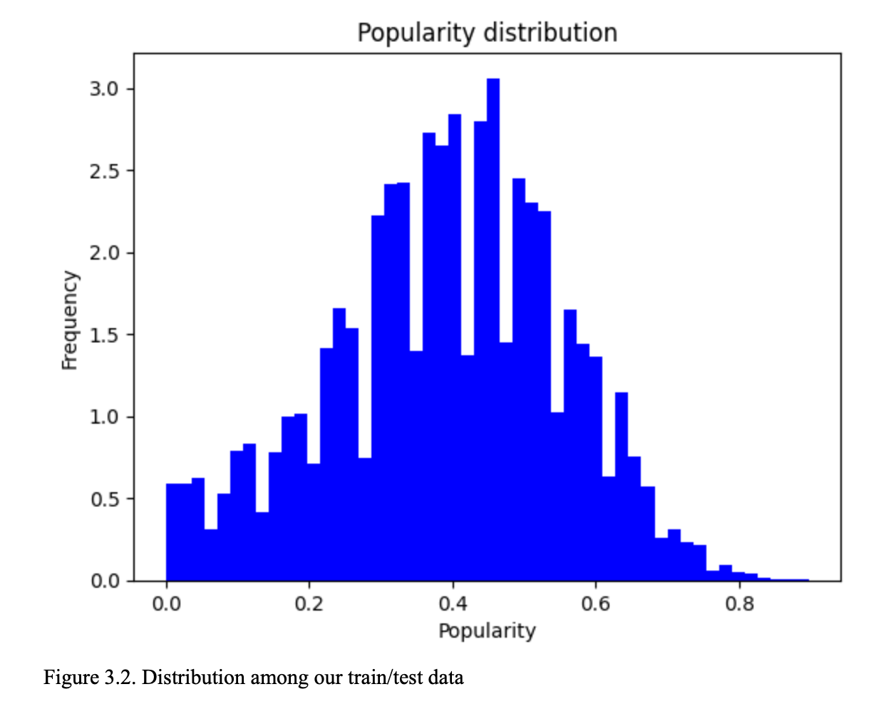
Additionally, as can be seen in figure 3.2, the target’s distribution is condensed at a central point, and distributed in a Gaussian shape. To help our model accurately predict the shape of the results, we use multiply the losses by a weighting factor. This multiplication is important to make our model more likely to predict outliers. The equation is the following:
\begin{equation} \frac{1}{N} \sum_{i=1}^{N} \exp\left(\left(\frac_{i} - \text)}}{\alpha \cdot \text}\right)^2 \cdot \frac{1}{\beta}\right) \end{equation}
Our feed-forward network was suffering of vanishing gradients during training. To attempt to avoid this, we initialized all linear layers with a weight distributed by Xavier uniform, and a constant bias of 0.1.
Finding the Best Model
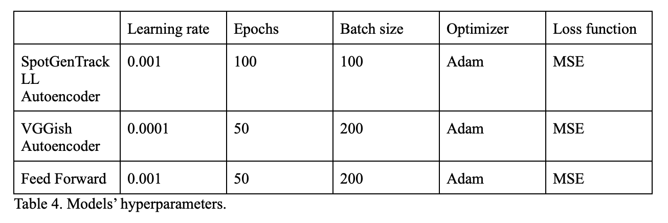
In order to find the best model, we modified plenty of parameters and hyperparameters. We first found the optimal autoencoder models (seen on table 4), and then we proceeded to run several loops over our linear layer to obtain the model with lowest errors. The parameters modified were the following:
- Learning rate: (0.001, 0.0001, 0.0002, 0.02, 0.0005)
- Weight decays: (0, 0.0001, 0.0002)
- Batch sizes: (200, 100, 256, 277)
- Means (for weights calculation): 0.33, 0.34, 0.35, 0.37, 0.38, 0.40, 0.42, 0.45)
- Alphas (for weights calculation): (1.8, 2.0, 2.1, 2.2)
- Betas (for weights calculation): (1.8, 2.0, 2.2)
- Number of linear layers: (7, 9, 12)
The combination that resulted in the optimal model was the following:
- Weight decays: 0
- Batch sizes: 200
- Means (for weights calculation): 0.36
- Alphas (for weights calculation): 2.0
- Betas (for weights calculation): 2.0

Table 5 shows the best-performing models obtained after experimentation. MAE, MSE and r-squared were calculated using the testing data, i.e. Data not used in training. Looking at the data in tables 2 and 3, we see that our model shows a significant improvement above the random baseline, with a reasonable r-squared and MSE. Reduction in the MAE remains challenging, but still we see a significant improvement from the random baseline.
Furthermore, we analyzed the testing data, and found that in 919 of the 1,500 songs (61.2%) of the songs, our model did better than HitMusicNet. Upon further analysis, we found that our model did a better job predicting the popularity of songs with popularities ranged [0.22-0.55], while HMN does a better job at predicting outliers (songs with <0.2 or >0.6 of popularity).
Conclusions and Next Steps
Data Exploration
Given Spotify’s ubiquity and analytics excellence, its Popularity Index is a good proxy for relative song popularity. But there are concerns around using data from a single platform (Spotify) and from a single channel (digital streaming). Given this concern, we would like to explore other methods of calibrating a track’s popularity (for example, Billboard and Discogs API). We can aggregate popularities into a single output, or can train each model on multiple outputs of various popularity scores.
Currently, our data consists of 30s audio clips. The average new song length is around 3min 17s, meaning that our models’ inputs cover around 15% of the song. This can cause the model to miss information critical to song likeability, such as the intro, chorus, or bridge. We would like to make our dataset more complete by using full songs as inputs. Furthermore, we’re using only 10,000 data points, which can also be affecting our training efficiency, especially our ability to detect outliers, which we have found to be a key issue with our model. Ideally, we would like to train our models on all 95k songs in SpotGenTrack.
Architectures
Many more architectures can further be explored to predict song popularity. We found VGGish with an LSTM to be an efficient “boosting” algorithm, which contributed to the model in a less significant way that SpotGenTrack, but still allowed our model to increase its performance. Similarly, the use of transformer architectures can help improve the performance of our model.
In this study, we explored and evaluated our model against the HitMusicNet’s regression algorithm. In further studies, it could be beneficial to explore the classification algorithm, as we have seen very promising results in the prediction of songs along a certain range.
We used the VGGish model purely on inference since we required to train the autoencoder and then the feed-forward network. Future studies can include architectures such that the VGGish model is trained in series with the feedforward network, and fine-tuned to predict popularity. We could also look at alternate representation models that are perhaps better suited or supply a more apt representation for our task than VGGish.
In conclusion, the use of low-level features to predict popularity can have several real-world advantages. The proposed model is able to predict a song’s popularity to a fair degree without the need for high-level features. Emerging artists can use these parameters to determine the possible success of their songs. Music labels can use this algorithm to predict an artist’s possible popularity. Platforms such as Spotify can also take advantage of this model in order to tackle recommendations and boost emerging artists.
Bibliography
- D. Martín-Gutiérrez, G. Hernández Peñaloza, A. Belmonte-Hernández and F. Álvarez García, “A Multimodal End-to-End Deep Learning Architecture for Music Popularity Prediction,” in IEEE Access, vol. 8, pp. 39361-39374, 2020, doi: 10.1109/ACCESS.2020.2976033.
- Ding, Yiwei, and Alexander Lerch. “Audio embeddings as teachers for music classification.” arXiv preprint arXiv:2306.17424 (2023).
- D. Martín-Gutiérrez, “HitMusicNet” in https://github.com/dmgutierrez/hitmusicnet.
- Koutini, Khaled, et al. “Efficient training of audio transformers with patchout.” arXiv preprint arXiv:2110.05069 (2021).
- P. Nandi, “Recurrent Neural Nets for Audio Classification” in https://towardsdatascience.com/recurrent-neural-nets-for-audio-classification-81cb62327990.
- Wu, Rick, “VGGish Tensorflow to PyTorch” in https://github.com/tcvrick/audioset-vggish-tensorflow-to-pytorch.
- Wu, Yiming. (2023). Self-Supervised Disentanglement of Harmonic and Rhythmic Features in Music Audio Signals.
- S. Shahane, “Spotify and Genius Track Dataset” in https://www.kaggle.com/datasets/saurabhshahane/spotgen-music-dataset/data.