How does model size impact catastrophic forgetting in online continual learning?

Yes, model size matters.

Introduction

One of the biggest unsolved challenges in continual learning is preventing forgetting previously learned information upon acquiring new information. Known as “catastrophic forgetting,” this phenomenon is particularly pertinent in scenarios where AI systems must adapt to new data without losing valuable insights from past experiences. Numerous studies have investigated different approaches to solving this problem in the past years, mostly around proposing innovative strategies to modify the way models are trained and measuring its impact on model performance, such as accuracy and forgetting.

Yet, compared to the numerous amount of studies done in establishing new strategies and evaluative approaches in visual continual learning, there is surprisingly little discussion on the impact of model size. It is commonly known that the size of a deep learning model (the number of parameters) is known to play a crucial role in its learning capabilities . Given the limitations in computational resources in most real-world circumstances, it is often not practical or feasible to choose the largest model available. In addition, sometimes smaller models perform just as well as larger models in specific contexts. Given this context, a better understanding of how model size impacts performance in a continual learning setting can provide insights and implications on real-world deployment of continual learning systems.

In this blog post, I explore the following research question: How do network depth and width impact model performance in an online continual learning setting? I set forth a hypothesis based on existing literature and conduct a series experiments with models of varying sizes to explore this relationship. This study aims to shed light on whether larger models truly offer an advantage in mitigating catastrophic forgetting, or if the reality is more nuanced.

Online continual learning

Continual learning (CL), also known as lifelong learning or incremental learning, is an approach that seeks to continually learn from non-iid data streams without forgetting previously acquired knowledge. The challenge in continual learning is generally known as the stability-plasticity dilemma, and the goal of continual learning is to strike a balance between learning stability and plasticity.

While traditional CL models assume new data arrives task by task, each with a stable data distribution, enabling offline training. However, this requires having access to all task data, which can be impractical due to privacy or resource limitations. In this study, I will consider a more realistic setting of Online Continual Learning (OCL), where data arrives in smaller batches and are not accessible after training, requiring models to learn from a single pass over an online data stream. This allows the model to learn data in real-time.

Online continual learning can involve adapting to new classes (class-incremental) or changing data characteristics (domain-incremental). Specifically, for class-incremental learning, the goal is to continually expand the model’s ability to recognize an increasing number of classes, maintaining its performance on all classes it has seen so far, despite not having continued access to the old class data. Moreover, there has been more recent work done in unsupervised continual learning . To narrow the scope of the vast CL landscape to focus on learning the impact of model size in CL performance, I will focus on the more common problem of class-incremental learning in supervised image classification in this study.

Continual learning techniques

Popular methods to mitigate catastrophic forgetting in continual learning generally fall into three buckets: :

regularization-based approaches that modify the classification objective to preserve past representations or foster more insightful representations, such as Elastic Weight Consolidation (EWC) and Learning without Forgetting (LwF);
memory-based approaches that replay samples retrieved from a memory buffer along with every incoming mini-batch, including Experience Replay (ER) and Maximally Interfered Retrieval, with variations on how the memory is retrieved and how the model and memory are updated; and
architectural approaches including parameter-isolation approaches where new parameters are added for new tasks and leaving previous parameters unchanged such as Progressive Neural Networks (PNNs).

Moreover, there are many methods that combine two or more of these techniques such as Averaged Gradient Episodic Memory (A-GEM) and Incremental Classifier and Representation Learning (iCaRL).

Among the methods, Experience Replay (ER) is a classic replay-based method and widely used for online continual learning. Despite its simplicity, recent studies have shown ER still outperforms many of the newer methods that have come after that, especially for online continual learning .

Model size and performance

It is generally known across literature that deeper models increase performance. Bianco et al. conducted a survey of key performance-related metrics to compare across various architectures, including accuracy, model complexity, computational complexity, and accuracy density. Relationship between model width and performance is also been discussed, albeit less frequently.

He et al. introduced Residual Networks (ResNets) which was a major innovation in computer vision by tackling the problem of degradation in deeper networks. ResNets do this by residual blocks to increase the accuracy of deeper models. Residual blocks that contain two ore more layers are stacked together, and “skip connections” are used in between these blocks. The skip connections act as an alternate shortcut for the gradient to pass through, which alleviates the issue of vanishing gradient. They also make it easier for the model to learn identity functions. As a result, ResNet improves the efficiency of deep neural networks with more neural layers while minimizing the percentage of errors. The authors compare models of different depths (composed of 18, 34, 50, 101, 152 layers) and show that accuracy increases with depth of the model.

	ResNet18	ResNet34	ResNet50	ResNet101	ResNet152
Number of Layers	18	34	50	101	152
Number of Parameters	~11.7 million	~21.8 million	~25.6 million	~44.5 million	~60 million
Top-1 Accuracy	69.76%	73.31%	76.13%	77.37%	78.31%
Top-5 Accuracy	89.08%	91.42%	92.86%	93.68%	94.05%
FLOPs	1.8 billion	3.6 billion	3.8 billion	7.6 billion	11.3 billion

Table 1: Comparison of ResNet Architectures

This leads to the question: do larger models perform better in continual learning? While much of the focus in continual learning research has often been on developing various strategies, methods, and establishing benchmarks, the impact of model scale remains a less explored path.

Moreover, recent studies on model scale in slightly different contexts have shown conflicting results. Luo et al. highlights a direct correlation between increasing model size and the severity of catastrophic forgetting in large language models (LLMs). They test models of varying sizes from 1 to 7 billion parameters. Yet, Dyer et al. show a constrasting perspective in the context of pretrained deep learning models. Their results show that large, pretrained ResNets and Transformers are a lot more resistant to forgetting than randomly-initialized, trained-from-scratch models, and that this tendency increases with the scale of model and the pretraining dataset size.

The relative lack of discussion on model size and the conflicting perspectives among existing studies indicate that the answer to the question is far from being definitive. In the next section, I will describe further how I approach this study.

Method

Problem definition

Online continual learning can be defined as follows:

The objective is to learn a function $f_\theta : \mathcal X \rightarrow \mathcal Y$ with parameters $\theta$ that predicts the label $Y \in \mathcal Y$ of the input $\mathbf X \in \mathcal X$. Over time steps $t \in \lbrace 1, 2, \ldots \infty \rbrace$, a distribution-varying stream $\mathcal S$ reveals data sequentially, which is different from classical supervised learning.

At every time step,

$\mathcal S$ reveals a set of data points (images) $\mathbf X_t \sim \pi_t$ from a non-stationary distribution $\pi_t$
Learner $f_\theta$ makes predictions $\hat Y_t$ based on current parameters $\theta_t$
$\mathcal S$ reveals true labels $Y_t$
Compare the predictions with the true labels, compute the training loss $L(Y_t, \hat Y_t)$
Learner updates the parameters of the model to $\theta_{t+1}$

Task-agnostic and boundary-agnostic

In the context of class-incremental learning, I will adopt the definitions of task-agnostic and boundary-agnostic from Soutif et al. 2023. A task-agnostic setting refers to when task labels are not available, which means the model does not know that the samples belong to a certain task. A boundary-agnostic setting is considered, where information on task boundaries are not available. This means that the model does not know when the data distribution changes to a new task.

	Yes	No
Task labels	Task-aware	Task-agnotic
Task boundaries	Boundary-aware	Boundary-agnostic

Table 2: Task labels and task boundaries. This project assumes task-agnostic and boundary-agnostic settings.

Experience Replay (ER)

In a class-incremental learning setting, the nature of the Experience Replay (ER) method aligns well with task-agnostic and boundary-agnostic settings. This is because ER focuses on replaying a subset of past experiences, which helps in maintaining knowledge of previous classes without needing explicit task labels or boundaries. This characteristic of ER allows it to adapt to new classes as they are introduced, while retaining the ability to recognize previously learned classes, making it inherently suitable for task-agnostic and boundary-agnostic continual learning scenarios.

Implementation-wise, ER involves randomly initializing an external memory buffer $\mathcal M$, then implementing before_training_exp and after_training_exp callbacks to use the dataloader to create mini-batches with samples from both training stream and the memory buffer. Each mini-batch is balanced so that all tasks or experiences are equally represented in terms of stored samples. As ER is known be well-suited for online continual learning, it will be the go-to method used to compare performances across models of varying sizes.

Benchmark

For this study, the SplitCIFAR-10 is used as the main benchmark. SplitCIFAR-10 splits the popular CIFAR-10 dataset into 5 tasks with disjoint classes, each task including 2 classes each. Each task has 10,000 3×32×32 images for training and 2000 images for testing. The model is exposed to these tasks or experiences sequentially, which simulates a real-world scenario where a learning system is exposed to new categories of data over time. This is suitable for class-incremental learning scenarios. This benchmark is used for both testing online and offline continual learning in this study.

Metrics

Key metrics established in earlier work in online continual learning are used to evaluate the performance of each model.

Average Anytime Accuracy (AAA) as defined in

The concept of average anytime accuracy serves as an indicator of a model’s overall performance throughout its learning phase, extending the idea of average incremental accuracy to include continuous assessment scenarios. This metric assesses the effectiveness of the model across all stages of training, rather than at a single endpoint, offering a more comprehensive view of its learning trajectory.

\[\text{AAA} = \frac{1}{T} \sum_{t=1}^{T} (\text{AA})_t\]

Average Cumulative Forgetting (ACF) as defined in

This equation represents the calculation of the Cumulative Accuracy ($b_k^t$) for task $k$ after the model has been trained up to task $t$. It computes the mean accuracy over the evaluation set $E^k_\Sigma$, which contains all instances $x$ and their true labels $y$ up to task $k$. The model’s prediction for each instance is given by $\underset{c \in C^k_\Sigma}{\text{arg max }} f^t(x)_c$, which selects the class $c$ with the highest predicted logit $f^t(x)_c$. The indicator function $1_y(\hat{y})$ outputs 1 if the prediction matches the true label, and 0 otherwise. The sum of these outputs is then averaged over the size of the evaluation set to compute the cumulative accuracy.

\[b_k^t = \frac{1}{|E^k_\Sigma|} \sum_{(x,y) \in E^k_\Sigma} 1_y(\underset{c \in C^k_\Sigma}{\text{arg max }} f^t(x)_c)\]

From Cumulative Accuracy, we can calculate the Average Cumulative Forgetting ($F_{\Sigma}^t$) by setting the cumulative forgetting about a previous cumulative task $k$, then averaging over all tasks learned so far:

\[F_{\Sigma}^t = \frac{1}{t-1} \sum_{k=1}^{t-1} \max_{i=1,...,t} \left( b_k^i - b_k^t \right)\]

Average Accuracy (AA) and Average Forgetting (AF) as defined in

$a_{i,j}$ is the accuracy evaluated on the test set of task $j$ after training the network from task 1 to $i$, while $i$ is the current task being trained. Average Accuracy (AA) is computed by averaging this over the number of tasks.

\[\text{Average Accuracy} (AA_i) = \frac{1}{i} \sum_{j=1}^{i} a_{i,j}\]

Average Forgetting measures how much a model’s performance on a previous task (task $j$) decreases after it has learned a new task (task $i$). It is calculated by comparing the highest accuracy the model $\max_{l \in {1, \ldots, k-1}} (a_{l, j})$ had on task $j$ before it learned task $k$, with the accuracy $a_{k, j}$ on task $j$ after learning task $k$.

\[\text{Average Forgetting}(F_i) = \frac{1}{i - 1} \sum_{j=1}^{i-1} f_{i,j}\] \[f_{k,j} = \max_{l \in \{1,...,k-1\}} (a_{l,j}) - a_{k,j}, \quad \forall j < k\]

In the context of class-incremental learning, the concept of classical forgetting may not provide meaningful insight due to its tendency to increase as the complexity of the task grows (considering more classes within the classification problem). Therefore, recommendeds avoiding relying on classical forgetting as a metric in settings of class-incremental learning, both online and offline settings. Thus, Average Anytime Accuracy (AAA) and Average Cumulative Forgetting (ACF) are used throughout this experiment, although AA and AF are computed as part of the process.

Model selection

To compare learning performance across varying model depths, I chose to use the popular ResNet architectures, particularly ResNet18, ResNet34, and ResNet50. As mentioned earlier in this blog, ResNets were designed to increase the performance of deeper neural networks, and their performance metrics are well known. While using custom models for more variability in sizes was a consideration, existing popular architectures were chosen for better reproducibility.

Moreover, while there are newer versions (i.e. ResNeXt) that have shown to perform better without a huge increase in computational complexity, for this study the original smaller models were chosen to avoid introducing unnecessary variables. ResNet18 and ResNet34 have the basic residual network structure, and ResNet50, ResNet101, and ResNet152 use slightly modified building blocks that have 3 layers instead of 2. This ”bottleneck design” was made to reduce training time. The specifics of the design of these models are detailed in the table from the original paper by He et al..

ResNet architecture. Table from He et al. (2015)

Moreover, in order to observe the effect of model width on performance, I also test a slim version of ResNet18 that has been used in previous works. The slim version uses fewer filters per layer, reducing the model width and computational load while keeping the original depth.

Saliency maps

I use saliency maps to visualize “attention” of the networks. Saliency maps are known to be useful for understanding which parts of the input image are most influential for the model’s predictions. By visualizing the specific areas of an image that a CNN considers important for classification, saliency maps provide insights into the internal representation and decision-making process of the network.

Experiment

The setup

Each model was trained from scratch using the Split-CIFAR10 benchmark with 2 classes per task, for 3 epoches with a mini-batch size of 64.
SGD optimizer with a 0.9 momentum and 1e-5 weight decay was used. The initial learning rate is set to 0.01 and the scheduler reduces it by a factor of 0.1 every 30 epochs, as done in .
Cross entropy loss is used as the criterion, as is common for image classification in continual learning.
Basic data augmentation is done on the training data to enhance model robustness and generalization by artificially expanding the dataset with varied, modified versions of the original images.
Each model is trained offline as well to serve as baselines.
Memory size of 500 is used to implement Experience Replay. This represents 1% of the training dataset.

Implementation

The continual learning benchmark was implemented using the Avalanche framework, an open source continual learning library, as well as the code for online continual learning by Soutif et al.. The experiments were run on Google Colab using NVIDIA Tesla T4 GPU.

	Experiment 1	Experiment 2	Experiment 3	Experiment 4	Experiment 5	Experiment 6	Experiment 7
Model	ResNet18	ResNet34	ResNet50	SlimResNet18	ResNet18	ResNet34	ResNet50
Strategy	Experience Replay	Experience Replay	Experience Replay	Experience Replay	Experience Replay	Experience Replay	Experience Replay
Benchmark	SplitCIFAR10	SplitCIFAR10	SplitCIFAR10	SplitCIFAR10	SplitCIFAR10	SplitCIFAR10	SplitCIFAR10
Training	Online	Online	Online	Online	Offline	Offline	Offline
GPU	V100	T4	A100	T4	T4	T4	T4
Training time (estimate)	3h	4.5h	5h	1h	<5m	<5m	<5m

Table 3: Details of experiments conducted in this study

Results

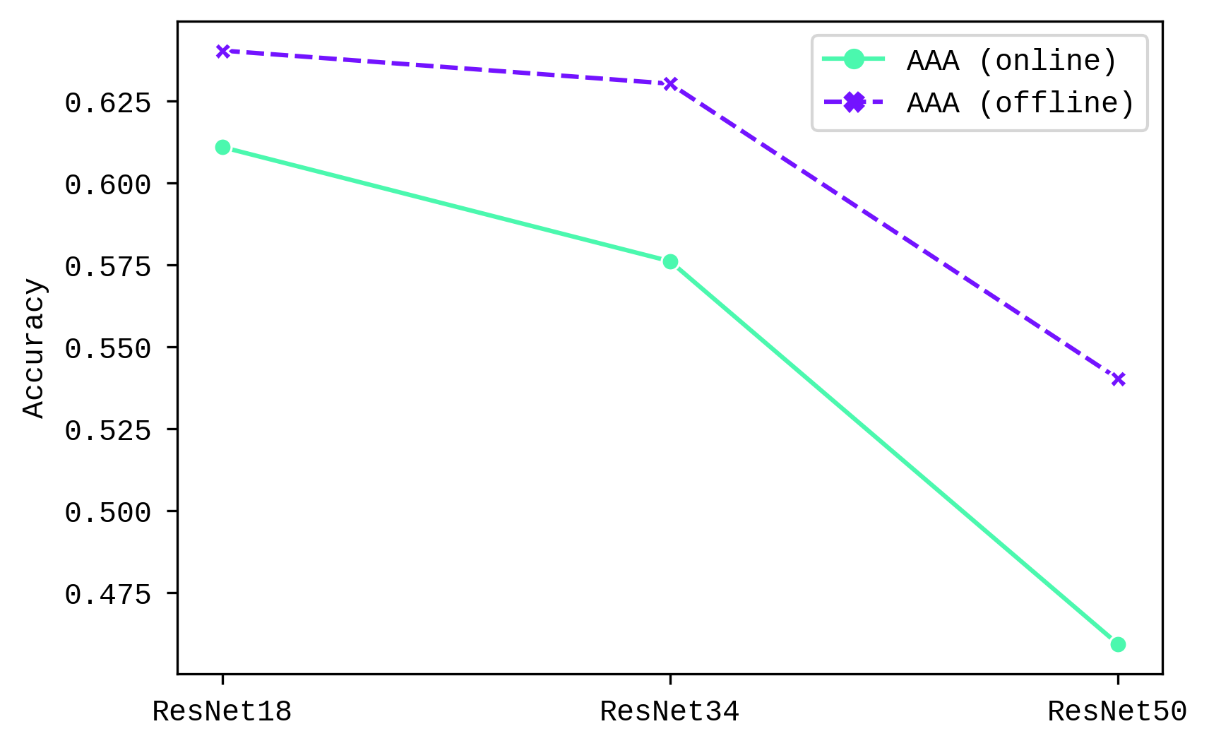
Average Anytime Accuracy (AAA) decreases with model size (Chart 1), with a sharper drop from ResNet34 to ResNet50. The decrease in AAA is more significant in online learning than offline learning.

Chart 1: Average Anytime Accuracy (AAA) of different sized ResNets in online and offline continual learning

When looking at average accuracy for validation stream for online CL setting (Chart 2), we see that the rate to which accuracy increases with each task degrade with larger models. Slim-ResNet18 shows the highest accuracy and growth trend. This could indicate that larger models are worse at generalizing to a class-incremental learning scenario.

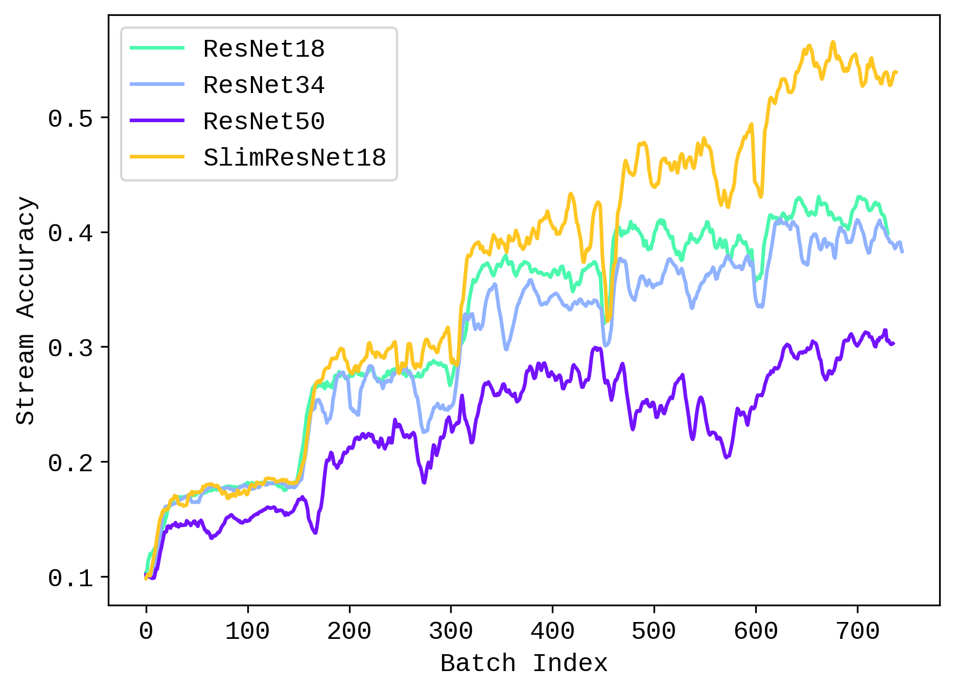
Chart 2: Validation stream accuracy (Online CL)

	Average Anytime Acc (AAA)	Final Average Acc
Slim ResNet18	0.664463	0.5364
ResNet18	0.610965	0.3712
ResNet34	0.576129	0.3568
ResNet50	0.459375	0.3036

Table 4: Accuracy metrics across differently sized models (Online CL)

Now we turn to forgetting.

Looking at Average Cumulative Forgetting (ACF), we see that for online CL setting, ResNet34 performs the best (with a slight overlap at the end with ResNet18), and ResNet50 shows the mosts forgetting. An noticeable observation in both ACF and AF is that ResNet50 performed better initially but forgetting started to increase after a few tasks.

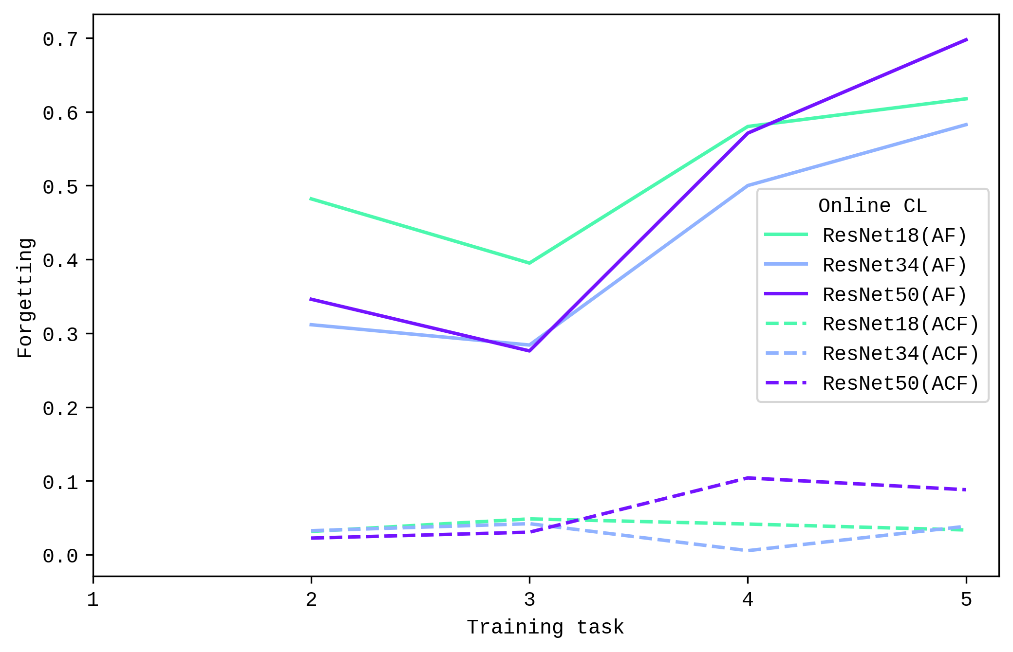
Chart 3: forgetting curves, Online CL (Solid: Average Forgetting (AF); Dotted: Average Cumulative Forgetting (ACF))

However, results look different for offline CL setting. ResNet50 has the lowest Average Cumulative Forgetting (ACF) (although with a slight increase in the middle), followed by ResNet18, and finally ResNet34. This differences in forgetting between online and offline CL setting is aligned with the accuracy metrics earlier, where the performance of ResNet50 decreases more starkly in the online CL setting.

Chart 4: Forgetting curves, Offline CL (Solid: Average Forgetting (AF); Dotted: Average Cumulative Forgetting (ACF))

Visual inspection of the saliency maps revealed some interesting observations. When it comes to the ability to highlight intuitive areas of interest in the images, there seemed to be a noticeable improvement from ResNet18 to ResNet34, but this was not necessarily the case from ResNet34 to ResNet50. This phenomenon was more salient in the online CL setting.

Online

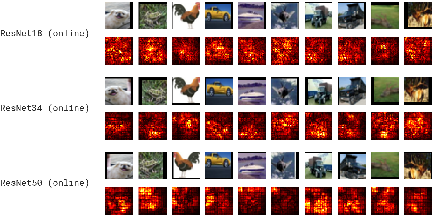
Offline

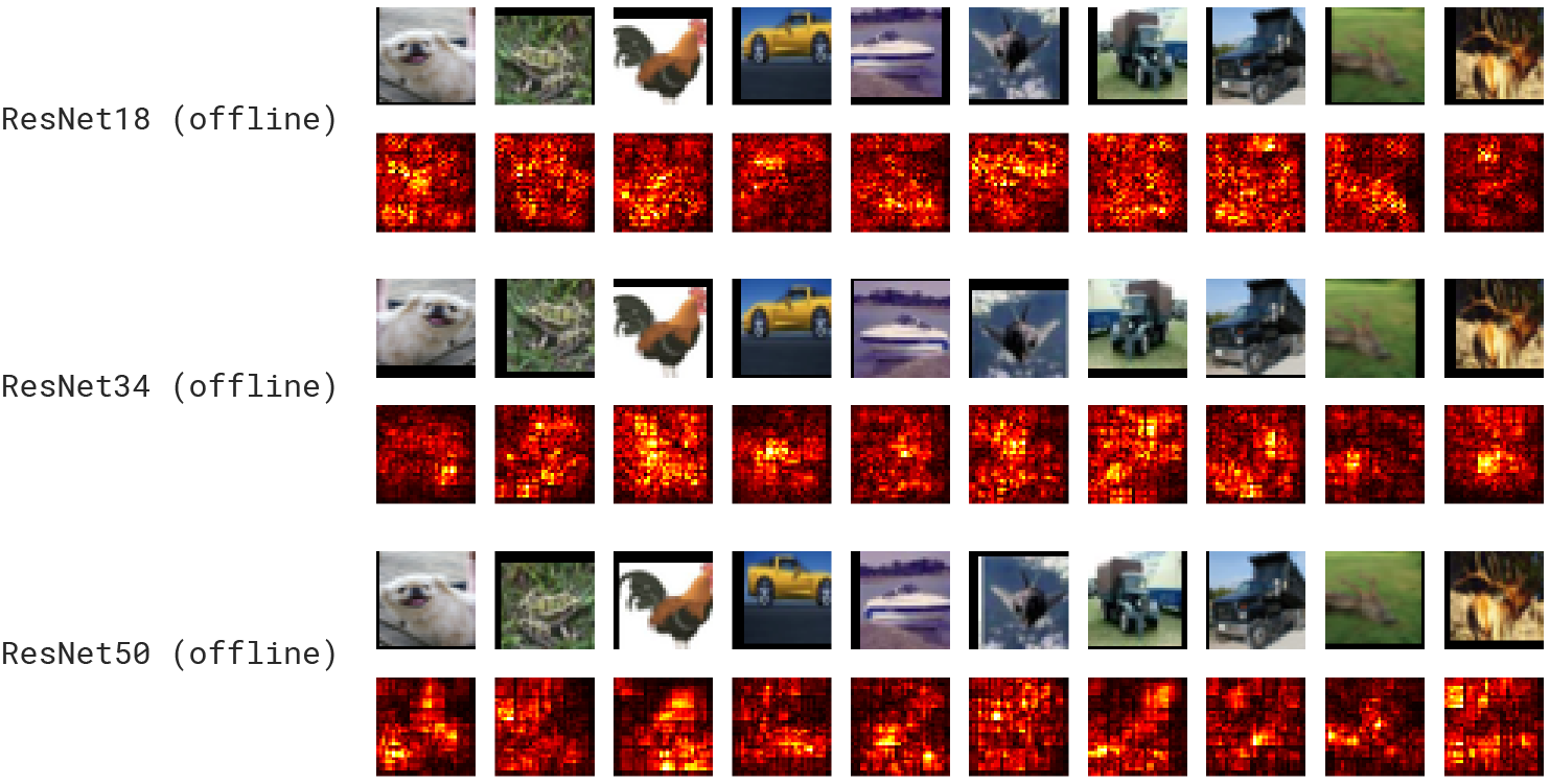
Interestingly, Slim-ResNet18 seems to be doing better than most of them, certainly better than its plain counterpart ResNet18. A further exploration of model width on performance and representation quality would be an interesting avenue of research.

Slim-ResNet18

Discussion

In this study, I compared key accuracy and forgetting metrics in online continual learning across ResNets of different depths and width, as well as brief qualitative inspection of the models’ internal representation. These results show that larger models do not necessary lead to better continual learning performance. We saw that Average Anytime Accuracy (AAA) and stream accuracy dropped progressively with model size, hinting that larger models struggle to generalize to newly trained tasks, especially in an online CL setting. Forgetting curves showed similar trends but with more nuance; larger models perform well at first but suffer from increased forgetting with more incoming tasks. Interestingly, the problem was not as pronounced in the offline CL setting, which highlights the challenges of training models in a more realistic, online continual learning context.

Why do larger models perform worse at continual learning? One of the reasons is that larger models tend to have more parameters, which might make it harder to maintain stability in the learned features as new data is introduced. This makes them more prone to overfitting and forgetting previously learned information, reducing their ability to generalize.

Building on this work, future research could investigate the impact of model size on CL performance by exploring the following questions:

Do pre-trained larger models (vs trained-from-scratch models) generalize better in continual learning settings?
Do longer training improve relatively performance of larger models in CL setting?
Can different CL strategies (other than Experience Replay) mitigate the degradation of performance in larger models?
Do slimmer versions of existing models always perform better?
How might different hyperparameters (i.e. learning rate) impact CL performance of larger models?

Conclusion

To conclude, this study has empirically explored the role of model size on performance in the context of online continual learning. Specifically, it has shown that model size matters when it comes to continual learning and forgetting, albeit in nuanced ways. These findings contribute to the ongoing discussions on the role of the scale of deep learning models on performance and have implications for future area of research.