Imposing uniformity through Poisson flow models

Uniformity and alignment are used to explain the success of contrastive encoders. Can we use already trained, well-aligned features and impose uniformity to increase their quality and performance on downstream classification tasks?

Most objects encountered in machine learning are extremely high dimensional. For example, a relatively small $512$x$512$ RGB image has over $750,000$ dimensions. However most of this space is empty, that is the set of well-formed images form an extremely small subset of this large space.

Thus a useful task in machine learning is to map this large space into a much smaller space, such that the images we care about form a compact organized distribution in this new space. This is called representation learning. For such a map to be useful, there are two key features. Firstly the representations should be useful for downstream tasks and not worse than the original representation. Thus they should preserve as much of the useful data as possible. Secondly, they should be relatively task agnostic and help across a diverse array of such downstream tasks. For example, word embeddings (such as those produced by BERT ) can be used for a wide array of language tasks such as language modeling and generation to sentiment analysis. An important question is how to generally find such useful representations.

Several methods exist. For example, autoencoders attempt to learn maps that are essentially bijective over the dataset we care about. These ensure that important information is not lost during the transformation. Contrastive encoders attempt to learn maps that enforce similarity between representations of similar images. Contrastive encoders are seen to perform quite well on unsupervised representation learning tasks, and we will explore these in a bit more detail soon. Lastly, we can layers of already trained neural networks can be used as features as well. For example, layers of VGG-19 trained on ImageNet are useful features that contain much information about the style and content of the images .

It is important to further quantify what makes a useful representation from a theoretical standpoint. Wang and Isola introduced concepts of alignment and uniformity to explain why contrastive encoders perform well. Alignment is the idea that similar objects should have close feature vectors in the representation space. Uniformity is the idea that the set of well-formed objects should cover the representation space uniformly.

In this post, we will further examine how uniformity affects the quality of representations. To do this, we will use Poisson flows. As we shall see, Poisson flows are an incredibly useful tool to enforce uniformity. We show that enforcing uniformity on well-aligned features can improve representations as measured by their performance on downstream tasks.

Notation

We introduce several notations to make talking about representations easier. Let $\mathcal{X}$ be our original space of the data, and let $p_{\mathrm{x}}$ be the distribution of the data. Let $\mathcal{Y}$ be any representation space, and let $f: \mathcal{X} \to \mathcal{Y}$ be a mapping from the original space to the representation space. If $\mathrm{y} = f(\mathrm{x}), \ \mathrm{x} \sim p_{\mathrm{x}}$, then let $\mathrm{y} \sim p_{f}$ and where $p_{f}$ is the new distribution after $f$.

We will also have a notion of similarity. Let $p_{\mathrm{pos}}(x_1, x_2)$ be a joint probability distribution that quantifies this similarity. We assume that $p_{\mathrm{pos}}$ satisfies

\[\begin{aligned} p_{\mathrm{pos}}(x_1, x_2) &= p_{\mathrm{pos}}(x_2, x_1) \\ \int_{x_2} p_{\mathrm{pos}}(x_1, x_2) d x_2 &= p_{\mathrm{x}}(x_1) \end{aligned}\]

Alignment and Uniformity

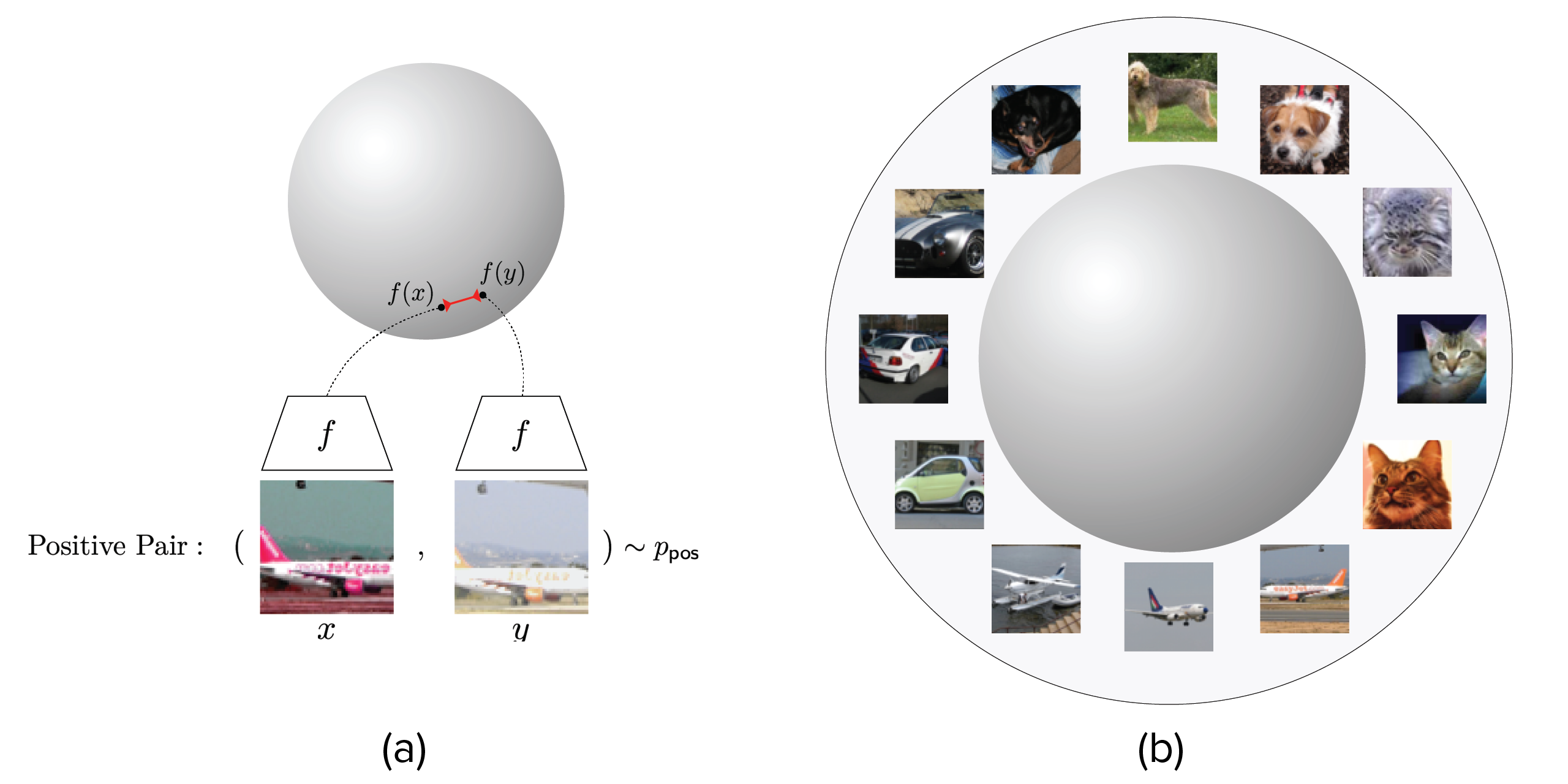
As mentioned earlier, contrastive autoencoders learn useful representations by minimizing a distance metric for similar pairs, while maximizing the same for dissimilar pairs . Thus if $D(x_1, x_2)$ is some distance metric of $\mathcal{Y}$, contrastive encoders maximize $d(x, x^+)$ for positive pairs, while minimizing $d(x, x^-)$ for negative pairs.

In their most common formulation, they set $\mathcal{Y}$ as the hypersphere $\mathcal{S}^d \subset \mathbb{R}^d$, and use cosine similarity $d(x_1, x_2) = x_1^T x_2$ as the similarity metric. Then the loss function becomes $M$ and $\tau$ are hyper parameters

\[\mathcal{L} \triangleq \mathbb{E}_{(x, x^+) \sim p_{\mathrm{pos}}, \{x_i^-\}_{i=1}^M \overset{\mathrm{iid}}{\sim} p_{\mathrm{x}}} \left[ \frac {e^{f(x)^T f(x^+)^T / \tau}} {e^{f(x)^T f(x^+)^T / \tau} + \sum_{i=1}^{M} e^{f(x)^T f(x_i^-)^T / \tau}} \right]\]

These encoders have been successful at several image representation tasks. Wang and Isola explained their performance through alignment and uniformity. Alignment, is simply the the quality that similar images are close together in the representation space. This is clearly present in contrastive encoders, as one of their goals is indeed to minimize

\[\mathcal{L}_{\mathrm{alignment}} \triangleq \mathbb{E}_{(x, x^+)\sim p_{\mathrm{pos}}} \left[ D(x, x^+) \right]\]

However, Wang and Isola also stated that uniformity was an equally important feature of contrastive architectures. That is, when training the contrastive loss to learn an encoder $f$, the new probability distribution $p_{f}$ is close to uniform. They showed that using $L_2$ norm as a distance metric and using Gaussian kernels to promote uniformity, learned representations perform better than those learned by contrastive learning.

Figure 1: Alignment and Uniformity. In figure (a), we see the quality of alignment, i.e. similar images are close to each other in the representation space. In figure (b), we see the quality of uniformity, i.e. images form a uniform distribution across the representation space. Image borrowed from

Why does uniformity help? Firstly, it acts as a regularization term. This is because if we tried to learn representations that maximized alignment without any target for uniformity, then a map that just takes all input vectors to zero would trivially minimize the loss. Yet this would be an extremely bad representation. However, aside from regularization, uniform distributions also have maximal self-entropy. Thus their importance can be explained equally well through some sort of minimizing loss of information. Indeed this is how explains it.

In this post we will investigate this even further. In particular, if regularization is the only effect that uniformity has on representations, then slightly nudging already aligned representations to make them uniform should not improve their quality. This is exactly what we will do, and we will do this through Poisson Flows.

Poisson Flows

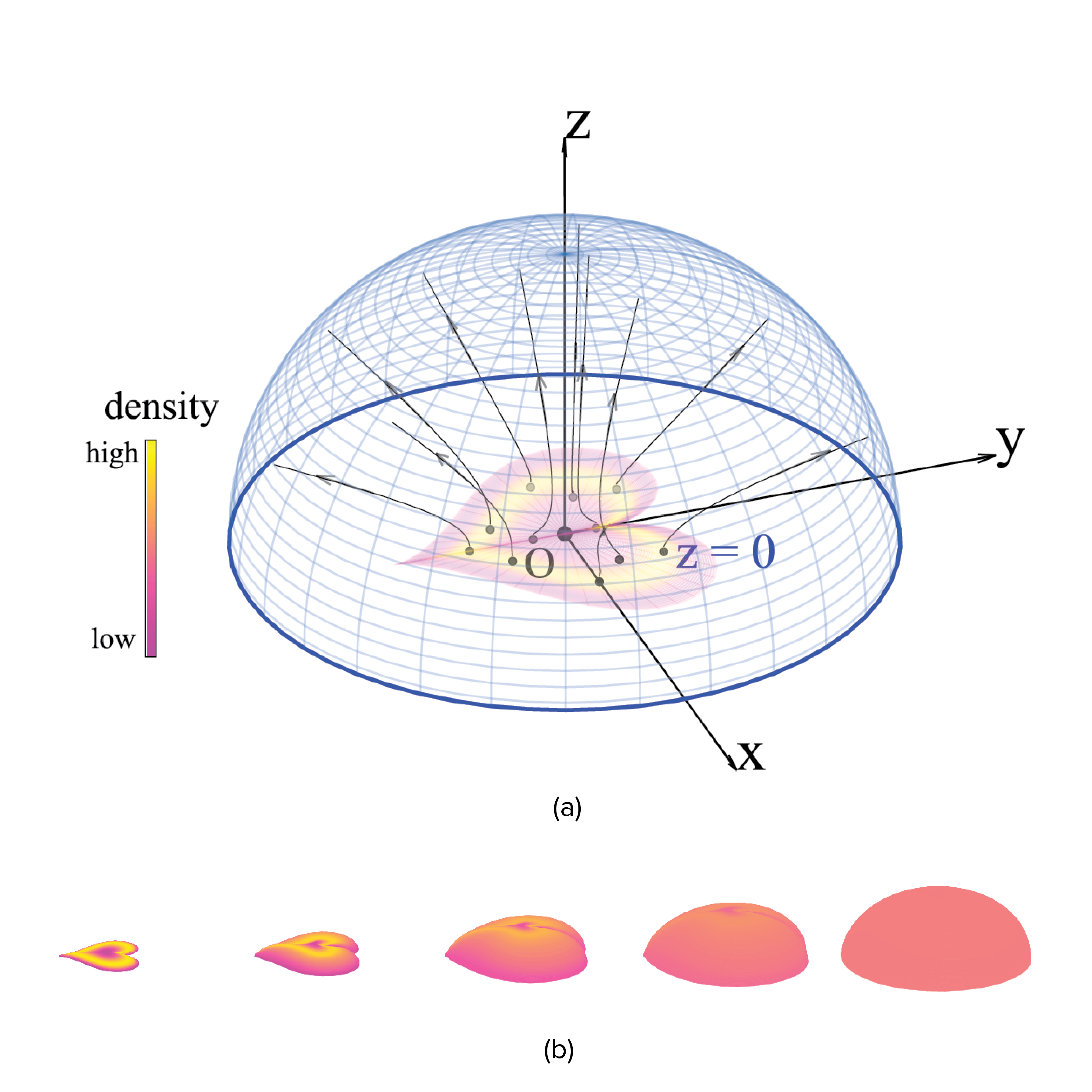
If you let a planar positive distribution of charges slightly above $z=0$ loose, then they will repel each other. If you stop them at some large enough distance $R$ from the origin, then their distribution approaches uniform as $R \to \infty$. This is very interesting, and what’s even more interesting is that this fact generalizes to arbitrary dimensions. Thus such fields allow a convenient way to map arbitrary high-dimensional distributions to uniform distributions. Poisson flow generative models proposed by Xu and Liu exploit this property for image generation; by sampling uniformly from the hemisphere, one can iterate through the backward ODE and thus sample from $p_{\mathrm{x}}$. We shall use it to impose uniformity on well-aligned features.

Figure 2: Evolution of data points through a Poisson field. As we can see, arbitrary distributions are mapped to uniform. Further the mapping is continuous. Borrowed from

Say we have a probability distribution $p_{\mathrm{y}}$ over $\mathcal{Y}_1 = \mathbb{R^d}$. Set this distribution at the $z = 0$ plane here z-dimension refers to the new dimension we recently augmented the dataset with in the expanded space $\tilde{\mathcal{Y}}_1 = \mathcal{Y} \times \mathbb{R}$. Let the electric field at an arbitrary point in $\tilde{\mathcal{Y}}_1$ be defined as

\[E_{p_{\tilde{\mathrm{y}}}}(\tilde{y}) = \int_{\tilde{y}'} \frac{\tilde{y} - \tilde{y'}}{\|\tilde{y} - \tilde{y'} \|_2^{d+1}} \cdot p_{\tilde{\mathrm{y}}}(\tilde{y}') d\tilde{y}'\]

Let $\mathrm{y} \sim p_{\mathrm{y}}$. Evolve $\tilde{\mathrm{y}} = (\mathrm{y}, 0) \in \tilde{\mathcal{Y}_1}$ according to the ODE

\[\frac{d\tilde{\mathrm{y}}}{dt} = E_{p_{\tilde{\mathrm{y}}}}(\tilde{y})\]

Let the final point be $f_{\mathrm{poisson}}(\mathrm{y}; p_{\mathrm{y}})$. Then the distribution of $p_{f_{\mathrm{poisson}}}(\cdot)$ approaches uniform as $R \to \infty$.

In practice, since we want to take $s = 0$ to $R$, we do a change of variables to write the ODE as

\[\frac{d \tilde{\mathrm{y}}}{ds} = \frac{1}{E_{p_{\tilde{\mathrm{y}}}}(\tilde{\mathrm{y}})^T \tilde{\mathrm{y}}} \cdot E_{p_{\tilde{\mathrm{y}}}}(\tilde{\mathrm{y}})\]

Note that the field stated here isn’t actually used directly, it is rather learned through a deep neural network. This is possible since the integral can be replaced with an expectation, which itself can be approximated through Monte-Carlo methods.

Since Poisson flows allow us to map arbitrary distributions to uniform ones, while preserving continuity; they are an extremely powerful tool to further understand the effects of uniformity. This brings us to our main hypothesis

Hypothesis

Assume that uniformity acts more than just a regularizing term for learning useful representations. Then if we take any well-aligned features that have good downstream performance, and apply a continuous map that imposes uniformity, our new features should perform better at downstream tasks

This is because if uniformity is simply a regularizing term, then training them for the downstream task is the best we can do. This hypothesis itself is counterintuitive because the original features should already be well-trained against the task at hand. However, surprisingly, this hypothesis seems to hold true. To show this, we describe the following experiment.

Experiment

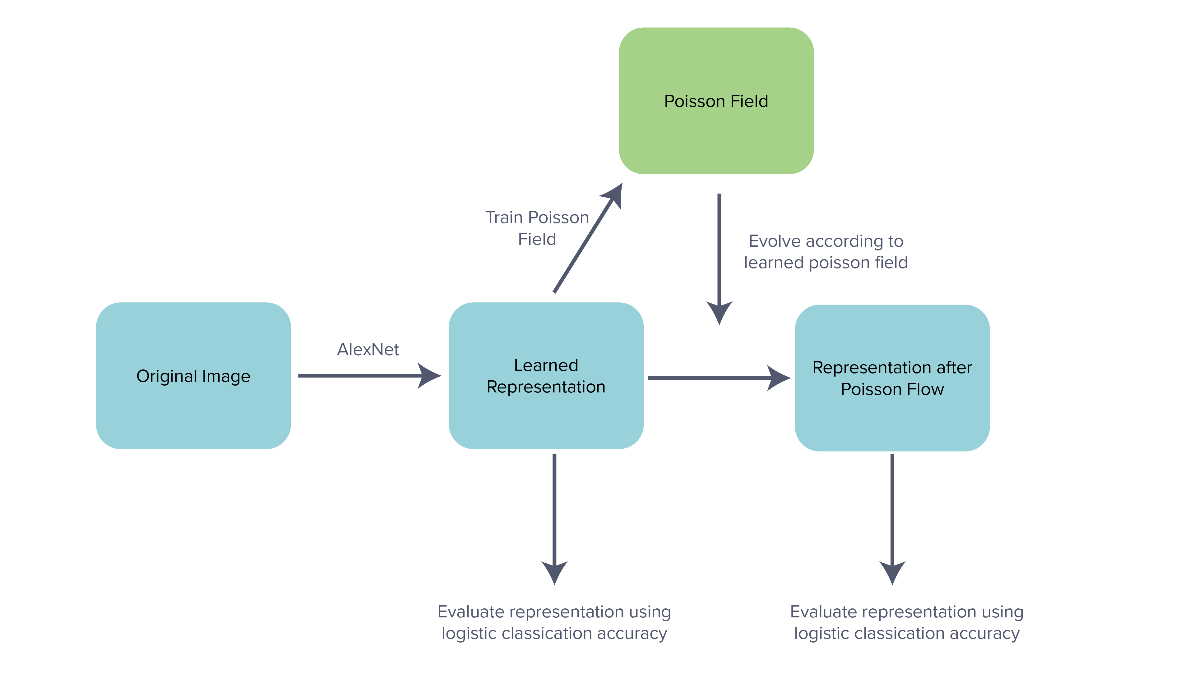
We consider the pen-ultimate layer of AlexNet trained on CIFAR-10 as our initial features. These features must be well aligned, as linear decision boundaries are able to accurately classify them into their classes.

Figure 3: A representation of how the features should evolve. (a) Initial representation is seemingly random and hard to classify with. (b) After training a classifier, the penultimate layer is well clustered between the various features. (c) Features after learning a Poisson field, and sending the data through it. Note that images (a) and (b) are for representation purposes only. However image (c) is indeed produced through a learned Poisson field from data points in (b)

We take these features and learn a corresponding Poisson field. For our predicted poisson field, we use a relatively small fixed-size two-hidden layer network.

We finally pass our features through this Poisson field and train a linear classifier on top of the final learned representations. We compare this accuracy against the original accuracy.

A summary of our approach is given in the figure below:

Figure 4: Overview of architecture

Further training details are given in Appendix A.

Results

The results are given in the below table.

Architecture	Train accuracy	Test accuracy
AlexNet	88%	82%
AlexNet + Poisson Flow (ours)	95%	85%

Here we see that our method outperforms a well-trained AlexNet considerably.

Conclusion

This is a surprisingly nice improvement. Note that the Poisson flow post-processing step is completely unsupervised. This seems to hint that having a uniform prior is helpful for reasons other than just regularization.

It would be extremely interesting to develop an entirely unsupervised architecture based on Poisson flow. This would begin by using an unsupervised method to learn well-aligned features. A suitable loss candidate could possibly be just a contrastive loss, with L2 norm as a distance metric:

\[\mathcal{L} \triangleq \mathbb{E}_{(x, x^+) \sim p_{\mathrm{pos}}, \{x_i^-\}_{i=1}^M \overset{\mathrm{iid}}{\sim} p_{\mathrm{x}}} \left[ \|x - x^+\|_2^{\alpha} - \lambda \sum_{i=1}^{M} \|x - x_i^{-}\|_2^{\beta} \right]\]

Then passing these well-aligned features through a Poisson flow would enforce uniformity. Such a proposed architecture could be worth exploring.

---

Appendices

See https://github.com/mathletema/poisson-representations for code.

Appendix A: Training details

We used a version of AlexNet similar to that given in Isola’s paper, such that the pen-ultimate layer was 128 neurons wide. We trained this network against cross entropy loss for 20 epochs using Adam as an optimizer.

After this, we moved the features from $\mathbb{R}^{128}$ to $\mathbb{R}^{129}$ by setting $z = 0$. We then learned a Poisson field for this network similar to . We use the default values of $\tau, \gamma, \sigma$ as the original paper, but used $M = 20$ as a consequence of our reduced dimension size. We trained this Poisson field with a large batch size of $1024$ and a small batch size of $128$. We trained this over $200$ epochs.

We then passed the features through the Poisson field. To simulate the ODE, we used Euler’s method with a small delta of $0.01$ and $100$ steps. Using RK4 might produce better results, and we leave this to future work.

We finally trained a logistic classifier on top of these final representations, and printed train and test accuracies.