Ensemble Learning for Mitigating Double Descent
Exploring when and why Double Descent occurs, and how to mitigate it through Ensemble Learning.
Abstract
We outline the fundamental ‘bias-variance tradeoff’ concept in machine learning, as well as how the double descent phenomenon counterintuitively bucks this trend for models with levels of parameterization at or beyond the number of data points in a training set. We present a novel investigation of the mitigation of the double descent phenomenon by coupling overparameterized neural networks with each other as well as various weak learners. Our findings demonstrate that coupling neural models results in decreased loss during the variance-induced jump in loss before the interpolation threshold, as well as a considerable improvement in model performance well past this threshold. Machine learning practitioners may also find useful the additional dimension of parallelization allowed through ensemble training when invoking double descent.
Motivation
There are many important considerations that machine learning scientists and engineers must consider when developing a model. How long should I train a model for? What features and data should I focus on? What exactly is an appropriate model size? This last question is a particularly interesting one, as there is a bit of contention regarding the correct answer between different schools of thought. A classical statistician may argue that, at a certain point, larger models begin to hurt our ability to generalize. By adding more and more parameters, we may end up overfitting to the training data, resulting in a model that poorly generalizes on new samples. On the other hand, a modern machine learning scientist may contest that a bigger model is always better. If the true function relating an input and output is conveyed by a simple function, in reality, neither of these ideas are completely correct in practice, and empirical findings demonstrate some combination of these philosophies. This brings us to the concept known as double descent. Double descent is the phenomenon where, as a model’s size is increased, test loss increases after reaching a minimum, then eventually decreases again, potentially to a new global minimum. This often happens in the region where training loss becomes zero (or whatever the ’perfect’ loss score may be), which can be interpreted as the model ’memorizing’ the training data given to it. Miraculously, however, the model is not only memorizing the training data, but learning to generalize as well, as is indicated by the decreasing test loss.
The question of ’how big should my model be?’ is key to the studies of machine learning practitioners. While many over-parameterized models can achieve lower test losses than the initial test loss minimum, it is fair to ask if the additional time, computing resources, and electricity used make the additional performance worth it. To study this question in a novel way, we propose incorporating ensemble learning.
Ensemble learning is the practice of using several machine learning models in conjunction to potentially achieve even greater accuracy on test datasets than any of the individual models. Ensemble learning is quite popular for classification tasks due to this reduced error empirically found on many datasets. To our knowledge, there is not much literature on how double descent is affected by ensemble learning versus how the phenomenon arises for any individual model.
We are effectively studying two different types of model complexity: one that incorporates higher levels of parameterization for an individual model, and one that uses several models in conjunction with each other. We demonstrate how ensemble learning affects the onset of the double descent phenomenon. By creating an ensemble that includes (or is fully comprised of) overparameterized neural networks, which can take extreme amounts of time and resources to generate, with overparameterized machine learning models, we will show the changes in the loss curve, specifically noting the changes in the regions where double descent is invoked. We hope that the results we have found can potentially be used by machine learning researchers and engineers to build more effective models.
Related Work
One of the first papers discussing double descent was ’Reconciling modern machine- learning practice and the classical bias–variance trade-off’ by Belkin et al.
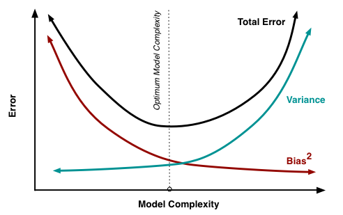
In short, classical statistical learning argues that there is some optimal level of parameterization of a model, where it is neither underparameterized nor overparameterized, that minimizes the total error between bias and variance. However, Belkin’s paper finds that, empirically, the tension between bias and variance no longer becomes a tradeoff after a certain level of overparamaterization. They showed that after the interpolation threshold (beyond where the model fits perfectly to the training data), test error eventually began to decrease again, even going below the error deemed optimal by the bias-variance minimum.
Nakkiran et al.’s ’Deep Double Descent: Where Bigger Models and More Data Hurt’

For the region between the first and second loss minima, model performance can suffer greatly, despite the increased computational time and resources used to generate such models. While this region of the test loss curve is typically not a level of parameterization that one would use in practice, understanding such loss curve behavior can help practitioners for several reasons. For one, this degraded phase of performance can be crucial for tweaking model architecture and adjusting training strategies. This is key to discovering if one’s model is robust and adaptable to various other datasets and tasks. This highlights the need for a new understanding for model selection in order to effectively generalize to testing datasets better, mitigating decreases in model performance and invoking a second loss minimum quickly.
In the classic paper ’Bagging Predictors’, Breiman describes the concept of combining the decisions of multiple models to improve classification ability
Setup
Computing Resources and Software
We have implemented this project using CUDA and the free version of Google Colab, with additional computing units for more costly experiments. To train and test these models, we use various machine learning packages in Python, namely Scikit-learn, PyTorch and Tensorflow. Additional software commonly used for machine learning projects, such as numpy, tensorboard and matplotlib, was also utilized.
All plots have been produced by us, unless otherwise specified. Note that all tensorboard plots have $0.25$ smoothing applied, except for the Soft-Voting Ensemble, which has $0.6$ smoothing applied (though this won’t make much of a difference as will soon be seen). The non-smoothed plot can be seen traced in light-blue in all provided plots.
Data
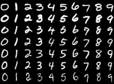
We use the MNIST dataset for this report
For this project, we use the MNIST dataset to unearth the double descent phenomenon. We experiment with a variety of models, as well as an ensemble of them: decision trees, AdaBoost trees, L2-Boost trees, random forests, logistic regression, and small neural networks. We choose these models because of their ability to be used for classification tasks, and more complicated models run the risk of exceeding Google Colab’s limitations, especially when we overparameterize these models to invoke double descent.
Models
Decision Trees
Decision trees are a machine learning model used for classification tasks. This model resembles a tree, splitting the data at branches, culminating in a prediction at the leaves of the tree.
To invoke overparameterization for decision trees, we can start with a tree of depth 2, and increase the number of maximum leaves of the model until the loss plateaus. Then, keeping this new number of max leaves in our decision tree, we continually increase the maximum depth of the tree until the loss once again stops decreasing. Lastly, keep both the maximum leaves and depth at their plateau levels while increasing the max features. The results of this are plotted below. Notice how varying the number of maximum leaves has minimal effect on the loss, and how increasing the maximum depth causes the most dramatic decrease. However, fluctuations on the maximum depth at this point do not have a major effect, whereas varying the number of features causes another slight, yet consistent, fall in classification loss.
Notice that the loss curve is more or less linear in the number of parameters (with some having much more effect than others), and so there is little evidence of double descent for this model.

AdaBoost Tree
Adaptive Boosting (AdaBoost) itself is an ensemble model used for robust classification. Freund et al.’s paper ‘A Decision-Theoretic Generalization of On-Line Learning and an Application to Boosting’ first introduced the algorithm
Notice that the loss curve is more or less linear in the number of parameters, and the double-U shape doesn’t seem to make its presence known.

L2-Boost Tree
L2 Boosting is quite similar to the AdaBoost model, except for L2 Boosting, as models are built sequentially, each new model in the boosting algorithm aims to minimize the L2 loss
Notice how the classification loss begins to fall, then rises up again, then falls once more when we average across more forests to lower minimums than before. This result was consistent across multiple runs of this experiment, suggesting that double descent is real for L2-Boosted Tree Ensembles.

The behavior of the loss once we add more models agrees with general intuition regarding ensembling, but the appearance of double descent as we increase the total number of parameters is still quite interesting to see. L2-Boost is a relatively inexpensive model and ensembling a large number of trees is still quite fast, suggesting that overparameterization could be the way to go in this case.
Random Forest
Random Forest is another popular ensemble model. As the name implies, it is a collection of decision trees with randomly selected features, and, like the singular decision tree, this model is used for classification tasks.
We initialize random forest with a small number of maximum leaves allowed in each tree, and increase the max leaves until we see the loss plateau as we continually add more. After this, we begin increasing the number of trees in our forest until the loss plateaus once again.
While Belkin et al. lists random forest as a model exhibiting double descent, this claim has been recently disputed, namely by Buschjager et al, which suggests that there is no true double descent with the random forest model
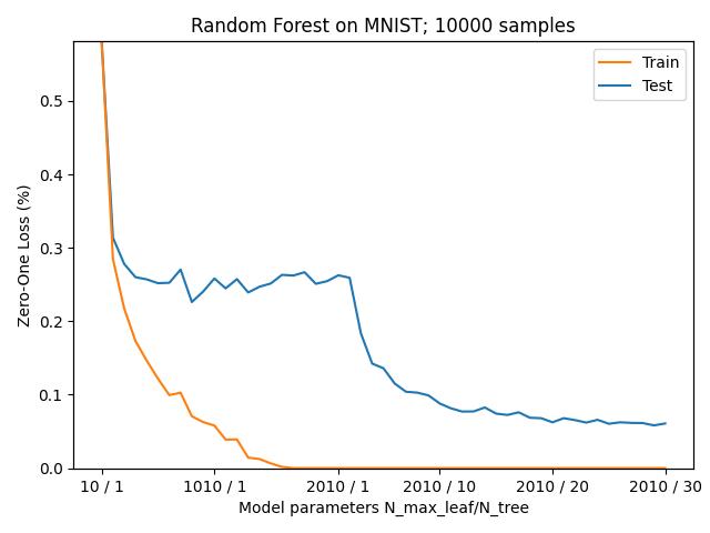
Despite this, for our ensemble model, we aim to see if the addition of this overparameterized learner to the neural network’s decision making is able to improve ensemble performance.
Logistic Regression
Logistic regression is a classic model used for estimating the probability a sample belongs to various classes. We induce overfitting in logistic regression through two methods.
First, we continually increase the ‘C’ parameter, indicating the inverse strength of regularization applied to the regression, as shown below. Notice that the loss decreases to a minimum before it starts slowly rising again, indicating that overfitting through fluctuations in ‘C’ may not actually lead to double descent, as would be expected from classical theory.

Second, we try inducing double descent by varying the ratio of the number of features over the amount of data. We gradually reduce this ratio using the intuition developed by Deng et al. in order to induce overfitting
To do this, we test varying across the number of training samples instead of varying the number of features used for training. This eventually leads to 0 training error, but causes testing error to blow up, suggesting that some significant amount of training data is still needed to witness the desired behavior, consistent with both statistical and machine learning theory.
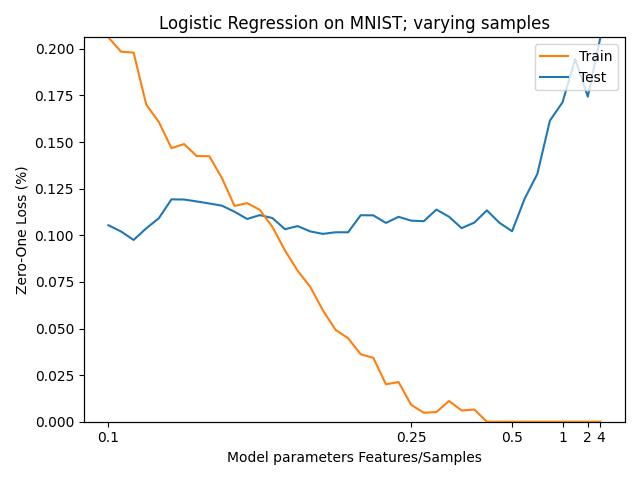
An interesting setup for future experiments would be simultaneously increasing the amount of training samples and the number of polynomial features given to the logistic regression, while increasing the feature-data ratio each time we reparameterize or redefine the dataset.
Neural Networks
We use a Multilayer Perceptron as our main model for the ensemble. Our deep learning model is a relatively small one, with variable width in the hidden layer. By increasing this width, we eventually achieve perfect training loss.
We define the general architecture of the neural network used in this report as follows:
Network Layer
Let the input data be an $m$ by $m$ pixel image from the MNIST dataset, which can be processed as an $m$ by $m$ matrix, where entry $(i,j)$ is an integer between $0$ and $255$ (inclusive) representing the grayscale color of the pixel. Note that $m=28$ for MNIST, though for generality, we use $ m $ in this network definition. A value of $0$ represents a black pixel, $255$ is a white pixel, and values between these are varying shades of gray. We first flatten this structure into a $d = m^2 $ by 1 vector, such that the entry $ (i,j) $ of the matrix becomes the $ j + 28*i$-th entry of the vector, using zero-indexing. We use this vector as the input of our neural network.
Set $H$ as the hidden layer width, which in our project will be varied in different tests. Let $ W^1 $ be an $ d \times H$ matrix, where $ W^1_{ij}$ is the weight of input $i$ applied to node $j$, and let $W^1_0$ be an $H \times 1$ column vector representing the biases added to the weighted input. For an input $X$, we define the pre-activation to be an $H \times 1$ vector represented by $Z = {W^1}^T X + W^1_0$.
We then pass this linearly transformed vector to the ReLU activation function, defined such that
\[\begin{equation*} \text{ReLU}(x)=\begin{cases} x \quad &\text{if} \, x > 0 \\ 0 \quad &\text{if} \, x \leq 0 \\ \end{cases} \end{equation*}\]We use this choice of activation function due to the well-known theorem of universal approximation. This theorem states that a feedforward network with at least one single hidden layer containing a finite number of neurons can approximate continuous functions on compact subsets of $ \mathbb{R}^{m^2} $ if the ReLU activation function is used
Next, we will input $A$ into a second hidden layer of the neural network. Let $K$ be the number of classes that the data can possibly belong to. Again, $K = 10$ for MNIST, though we will use $K$ for generality. Then let $W^2$ be an $H$ by $K$ matrix, where $W^2_{ij}$ is the weight of input $i$ applied to node $j$, and let $W^2_0$ be a $K \times 1$ column vector representing the biases added to the weighted input. For input $A$, define a second pre-activation to be a $K \times 1$ vector represented by $B = {W^2}^T A + W^2_0$.
This will yield a $K \times 1$ vector representing the logits of the input image, with which we’ll be able to take Cross Entropy Loss or compute its probability of belonging to any of the $K$ classes.
Training
Let class $i $ be the true classification for a data point. We have that $y_i = 1$, and for all $j \neq i$, $y_j = 0$. Furthermore, let $\hat{y_i}$ be the generated probability that the sample belongs to class $i$. The categorical cross-entropy loss is then defined as follows:
\[\mathcal{L}_{CCE} (y_i, \hat{y_i}) = - \sum_{i=0}^{9} y_i \log (\hat{y_i})\]From this computed loss, we use backpropagation and stochastic gradient descent (SGD) with learning rate $\eta = 0.1$ and $momentum = 0.95$ to optimize model weights. We run experiments on a dataset with $n = 4000$ subsamples that train over $100$, $500$, and $2000$ epochs using Belkin et al.’s approach to training
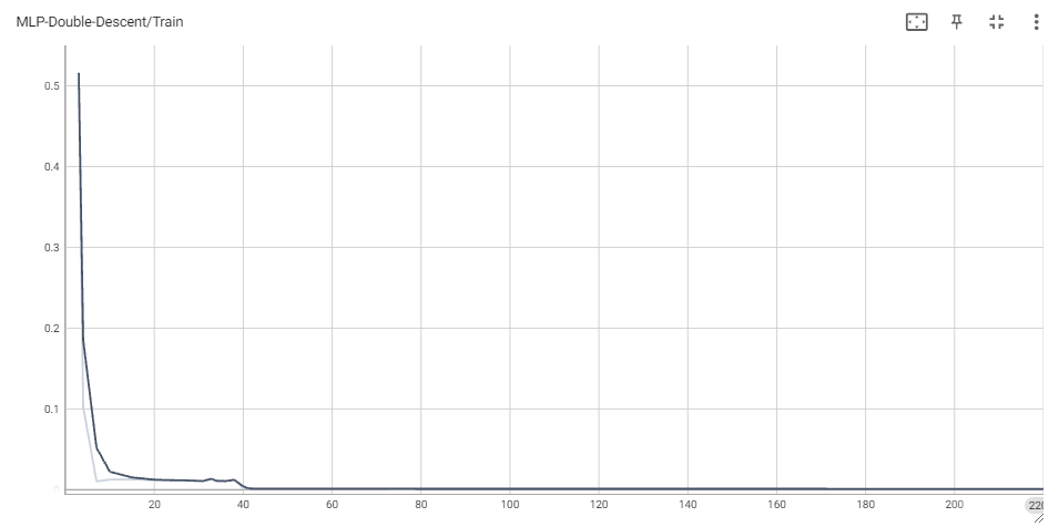
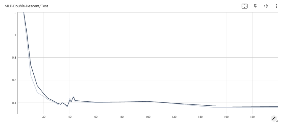
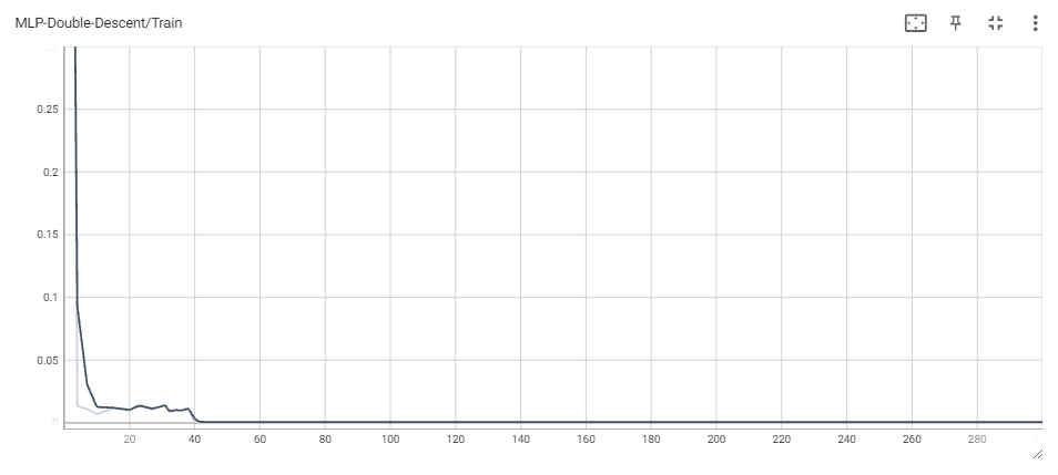
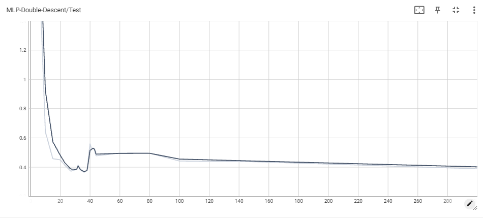
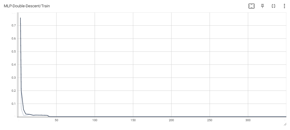
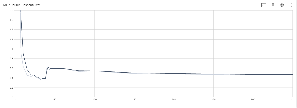
For the sake of brevity, we avoid including plots for train/test classification loss for the MLPs. However, it is worth noting that train classification loss eventually reaches 0 in all experiments, whereas test loss eventually becomes $\sim$ 0.08 or smaller.
Throughout each experiment, we vary across the number of total parameters of the model. For a network with $H$ hidden units, the total number of parameters is equal to $(d+1)\times H + (H + 1)\times K$, and so we choose $H$ accordingly each time we reparametrize.
Note that we also incorporated a weight reuse scheme for models in the underparametrized regime to cut on training time, similarly to the approach in Belkin et al
Additionally, even though the individual MLPs are small, training several of them sequentially for a relatively large number of epochs can take a very long time. To help reduce the time it takes to complete experiments, we also try adapting the Parameter Count Generation Algorithm provided in John Abascal’s blog
This algorithm proved helpful for empirically confirming the existence and validity of the interpolation threshold. However, after a few tests with the algorithm, we chose to complete most of the experiments using a pre-specified list of parameters which were able to consistently capture the double descent phenomena in detail.
Ensemble Learning
We experimented with two different types of ensembles. The first ensemble is what we call the ‘weak-learner’ ensemble, which is the model that incorporates the multi-layer perceptron supported by L2-Boost tree ensembles, random forests, decision trees and logistic regression. Note that we ultimately did not use AdaBoost in this ensemble because we believed this was too similar to the included L2-Boost model in both architecture and performance.
The second ensemble is the ‘multi-layer perceptron’ ensemble, which includes 5 MLPs.
Weak-Learner Ensemble
We use bootstrap aggregating, or ‘bagging’, to formulate our ensemble of these five models . Effectively, each model is given a certain number of ‘votes’ on what that model believes is the correct classification for any given MNIST sample image. We then experimented with two approaches to voting: hard voting and soft voting.
In hard voting, the classification with the most total votes is then used as the ensemble’s overall output. In the event of a tie, the neural network’s prediction is chosen. Using this voting scheme, we train the MLP independently of the other models in the ensemble, using the same scheme as described previously.
In soft voting, the weighted average of the predicted class probabilities of each model is used as the predicted class probabilities of the ensemble. We utilize this prediction when training the MLP, and use negative log likelihood loss instead of cross entropy loss, since taking the softmax of probabilities is not necessary. This way, we can incorporate the predictions of the whole ensemble into the training of the MLP. Since the ensemble now outputs a vector of class probabilities, the one with the highest probability will be used as the soft voting ensemble’s prediction.
Since we want a neural model to be the basis of our ensemble, we vary the number of votes assigned to the neural network while keeping the number of votes for other models fixed to 1. With four supplementary models in addition to the neural network, giving the neural network 4 or more votes is not necessary, since this ensemble would always output the same results as the neural network. Because of this, we study the loss curve when giving the neural network 1, 2, and 3 votes. Note that decimal value votes for the neural network are not sensible (at least in the hard-voting scheme), since it can be proved that all potential voting scenarios are encapsulated into the three voting levels we have chosen.
Another important aspect of our ensemble is that the ‘weak’ classifiers do not vary in parameterization; only the MLP does. Refitting all the weak classifiers across epochs and MLP parameterizations took much longer than expected, perhaps due to incompatibilities between sklearn and GPUs, and completing the experiments using this approach was unfortunately unfeasible. Hence, all ‘weak’ classifiers have fixed architectures, chosen such that each one has low test error but is not at the highest level of parameterization according to the previous discussion, and only the MLP varies.
Multi-Layer Perceptron Ensemble
The Multi-Layer Perceptron Ensemble uses 5 identically initialized MLPs which are trained in parallel using Pytorch’s autovectorization capabilities. Since they are defined in the same way and trained simultaneously using the MLP training scheme discussed above, each receives equal weight when it comes to taking an averaged prediction. However, unlike the bagging method used for the Weak-Learner Ensemble, we take advantage of the identical architectures of the models and the numerical stability provided by this, and generate ensemble predictions by averaging the logits of all five learners and using those values as the logits of the ensemble. Again, we experiment using 100 and 500 epochs to see how the behavior evolves across increasing number of epochs, but we omit training over 2000 epochs due to excessive computational costs. An experiment for the future would be training over a very large number of epochs for even greater ensemble sizes to see how results vary across time.
There has been discussion in the past of whether to average the raw logits or the softmax-transformed probabilities. The main concern raised over averaging across raw logits is that the outputted values can vary greatly in magnitude across models (and therefore overconfident models can potentially overshadow all other models when taking the prediction), but, empirically, that doesn’t seem to be a problem here. Tassi et al. provide some intuition in “The Impact of Averaging Logits Over Probabilities on Ensembles of Neural Networks”
Results and Discussion
Contrary to our expectations, the Weak Learner Ensemble performs much worse than even the individual models on MNIST classification. Although our focus is on double descent and not on the strong predictive power of ensembles, the latter is needed to observe the former, or at least discuss it at an interesting level.
Initially, we tried applying the soft-voting scheme for the Weak Learner Ensemble, but the reported results are unexpectedly poor, yielding very high classification loss, especially when compared to the results of each model taken individually. This may be because each ‘weak’ learner has high confidence in its predicted class, whereas the MLP may be more evenly split between different classes, which would result in the weak classifiers winning more often, even if the MLP has higher weight in the prediction. The plot of the negative log likelihood loss for both training and testing is also hard to understand, but it is clear the ensemble has a very hard time improving, even as more parameters are added. We only include the results for the ensemble that allocates 3 votes to the MLP, but note that these are the best loss curves we were able to produce given this method.
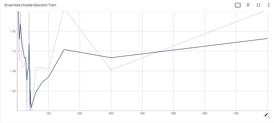
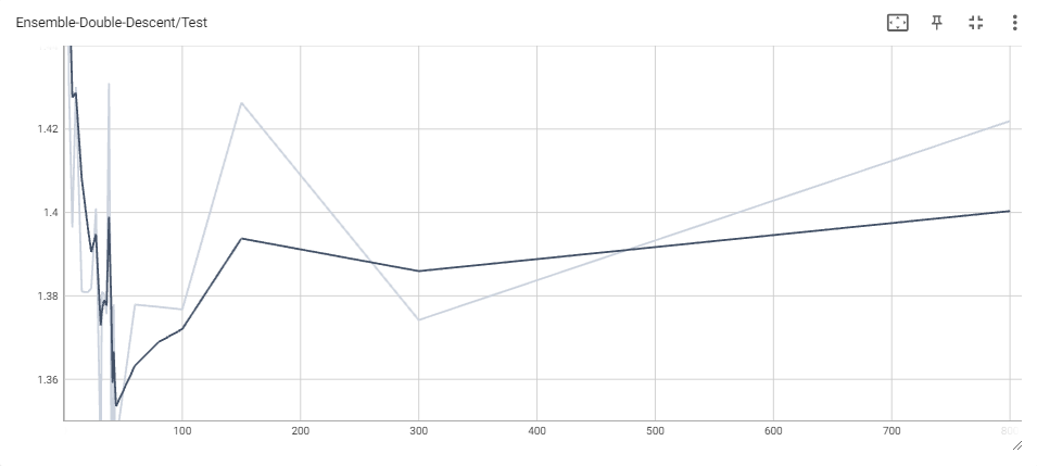
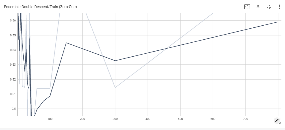
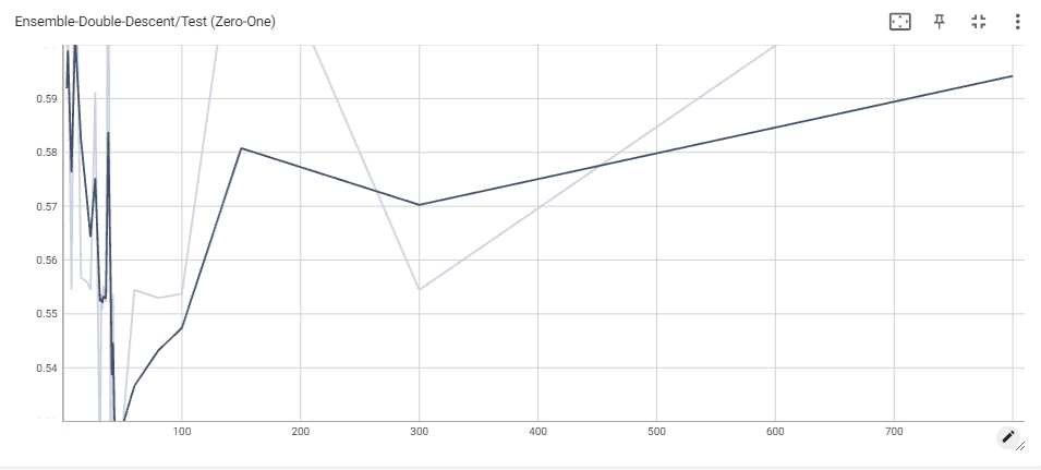
We then tried the weak-learner approach again with hard-voting, and let the MLP independently train using the unmodified MLP training scheme mentioned previously. However, as opposed to halting training when MLP classifications loss first hits 0, we only halt training when ensemble classification first hits 0.
We found that while classification loss had certainly gone down when compared to the soft-voting scheme (with even just one vote!), the ensemble still severely underperformed when compared to each of the individual models used. As seen in the plots, the classification loss starts to improve once the MLP gets more and more votes, agreeing with intuition that, eventually, the MLP has the veto right. As opposed to the soft-voting scheme, all classifiers now have a contribution that is proportional to their voting weight, which mitigates the previous problem of some models having much higher confidence than others. However, we believe the poor results can be attributed to the models we used for ensembling. Indeed, a significant number of models are regular, boosted or ensembled (or all) versions of decision trees, which means there is a significant chance that they make similar mistakes on similar data points. Looking at the plots for overparameterized decision trees and L2-Boost ensembles, we see that train error never quite reaches 0 for any of them. Since the train loss seems to pleateau for our models as well, this may prove why. In the cases of 1 or 2 votes, this can lead to consistently poor predictions, especially since the models are not reparameterized across the experiment. For 3 votes, this phenomenon is less significant, as the ensemble slowly begins to reach the testing performance of the individual models.

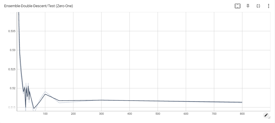
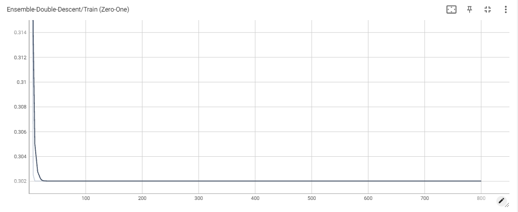
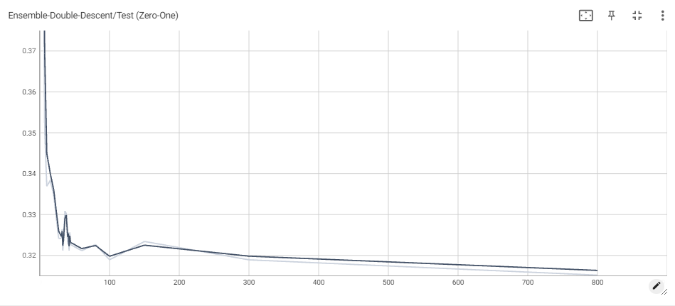
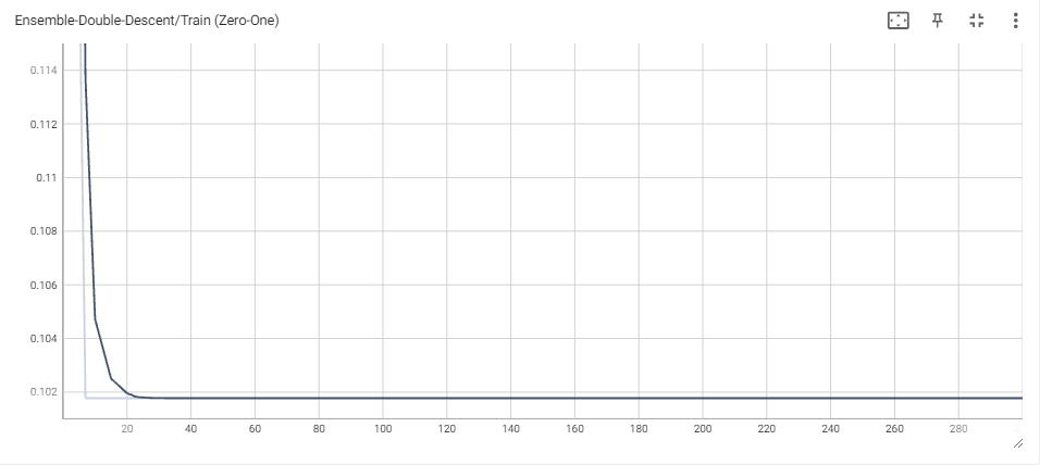
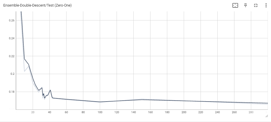
Further work could be done on the Weak-Learner Ensemble, focusing on better model selection and concurrent reparameterization across all models. Given the limited time and compute resources at our disposal, we leave this problem open for now.
All hope is not lost, however. Seeing the poor performance of the Weak-Learner Ensemble given the significantly better performance of individual models, one could be discouraged from attempting to use ensembling to mitigate double descent, since it may not even be observable in such settings. However, we saw double descent in L2-Boost ensembles and, arguably, in random forests, and so we pushed onward. All other ensemble methods used multiple copies of the same model, and so we decided to experiment with a small ensemble of MLPs, to see how they would behave.
This was feasible for 100 and 500 epochs only, but the obtained results shed light on how ensembling could in fact mitigate double descent. The phenomenon is not quite as observable in the 100 epoch case (one explanation could be that the train loss has not converged yet), but it becomes quite clear when looking at the 500 epoch ensemble and comparing it with the original 500 epoch MLP. Double descent is still very easy to see, ocuring at the same threshold as before. This makes sense, since the MLPs have all reached interpolation, which should increase test loss for all, and then start going down as we overparametrize more and more. However, the main result is that the increase once we reach interpolation is much lower than before. Indeed, the ensemble sees a jump from $\sim$ 0.35 to around $\sim$ 0.4 at the highest, whereas the individual MLP sees a jump from $\sim$ 0.36 to around $\sim$ 0.52. Another important result is that the loss as we overparameterize becomes significantly lower in the ensemble model than in the individual MLP.
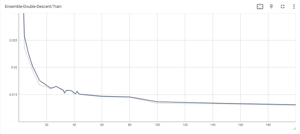
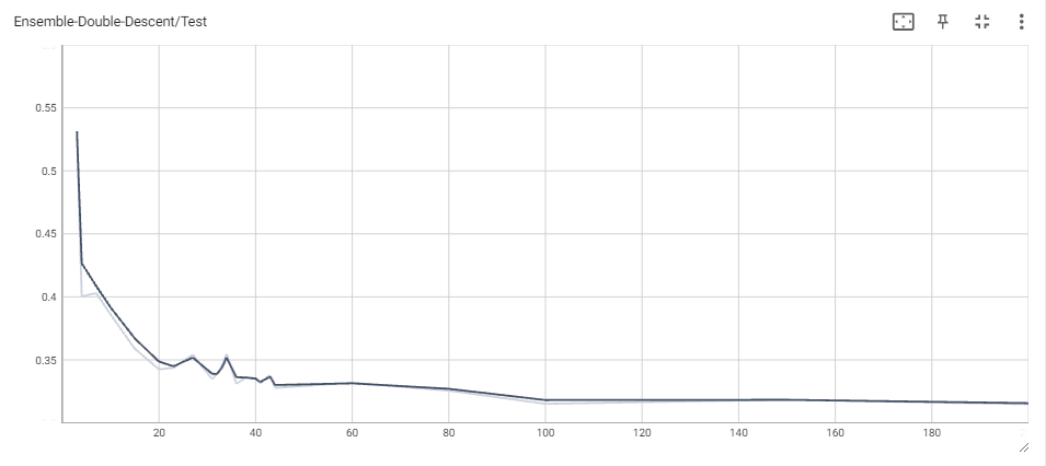
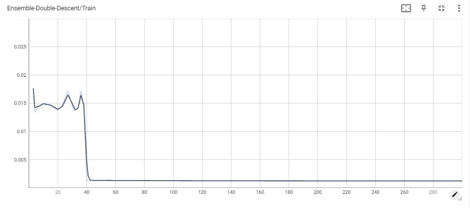
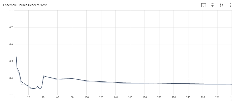
While we weren’t able to fully get rid of the double descent curve by ensembling multiple MLPs, the fact that it became flatter and the loss past the interpolation threshold started to become smaller is quite exciting, as it suggests that, potentially, large ensembles of MLPs may not noticeably suffer from double descent at all, and yield better overall predictions than individual models can. One notable advantage to this ensemble method is the ability to further parallelize one’s training of overparameterized neural networks. These models can take extreme lengths of time to train, and besides increasing the computational allocation used, practitioners may use data, model, or processor parallelism in order to reduce this time. The ensemble neural networks we use are independently generated, meaning that they can be vectorized or trained on different GPU cores without issue. This could be a valid alternative to training for more epochs for reducing model error past the interpolation threshold. More work investigating the effect of neural network ensembling on double descent, especially on models trained over many epochs, would be very exciting and potentially shed even more light on the possible advantages of overparameterization.
Conclusion
We discussed the existence of double descent for some simple and classical models, observing the effects of varying across levels of parameterization and noting that single descent can sometimes be mistaken for double descent, and proposed the use of various ensembles to mitigate the effects of double descent.
Ensembles consisting solely of neural networks resulted in a considerable boost in performance past the individual model interpolation threshold, and in a flatter curve when compared to individual models. However, pairing the neural network with weak learners in an ensemble voting system decreased testing performance, though this adverse effect waned as the neural network received proportionally more votes. Machine learning engineers that intend to intentionally overparameterize their models may take advantage of not only the ensemble approach’s increased performance and significantly more reliable results, but the enhanced parallelization and vectorization capabilities offered by the proposed method.
Future Work
This project was implemented using Google Colab, which proved to be restrictive for adopting more complex models. A key part of the double descent phenomenon is overparameterization, which happens across multiple full training loops, and so complex models that are additionally overparameterized will require more powerful computing resources beyond what we used. For example, a model which takes 10 hours to complete a single training loop will take multiple days to train before being able to plot results and observe double descent. Even for models that take around 10 to 15 minutes to train, such as the 500 epoch MLP we explored throughout our project, a full experiment that showcases the double descent curve in detail can take upwards of 5 hours. Furthermore, additional computing power can allow for this project to be expanded to more complicated datasets and tasks. MNIST classification is computationally inexpensive, though invoking double descent in more complex tasks such as text generation in natural language processing was not feasible using Google Colab. Future projects that follow this work should keep computational limitations in mind when choosing models and datasets.
In addition to the future work suggested throughout our project, we propose a final approach that we believe is worth exploring further. During the planning process of this project, we discussed using a more rigorous voting system than what is traditionally found in ensemble model projects. Effectively, each model would have a weight associated with how much influence its output should have on the overall ensemble output. For $n$ models, each model could start with, say, a weight of $1/n$. Then, after producing each model’s vector output, the categorical cross-entropy loss with respect the true output could be computed, and the weights of each model could be updated such that each model has its weight decreased by some amount proportional to the calculated loss. Then, these weights could be normalized using the softmax function. This would be repeated for each level of parameterization. Due to resource constraints and the limitations of sklearn to the CPU, learning both the model weights and ensemble weights at each level of ensemble parameterization was not feasible given the size of the models we built and the classifiers we chose to use, as well as the number of epochs we trained over. Future studies may wish to implement this method, however, to produce a more robust ensemble for classification.
Reproducibility Statement
To ensure reproducibility, we have included the codebase used for this project, as well as the above description of our data, models, and methods