6-DOF estimation through visual place recognition
A neural pose-estimation solution is implemented, which could help an agent with a downward-facing camera (such as a drone) to geolocate based on prior satellite imagery of terrain. The neural encoder infers extrinsic camera parameters from camera images, enabling estimation of 6 degrees of freedom (6-DOF), namely 3-space position and orientation. By encoding priors about satellite imagery in a neural network, the need for the agent to carry a satellite imagery dataset onboard is avoided.
Introduction
The goal of this project is to demonstrate how a drone or other platform with a downward-facing camera could perform approximate geolocation using a neural scene representation of existing satellite imagery. Note that the use of the term “Visual Place Recognition” in the title is a carryover from the proposal, but no longer applies to this project. Rather, the goal of this project is to implement 6-DOF pose-estimation.
Pose estimation
In this work, the goal is to compress the ground-truth image data into a neural model which maps live camera footage to geolocation coordinates.
Twitter user Stephan Sturges demonstrates his solution
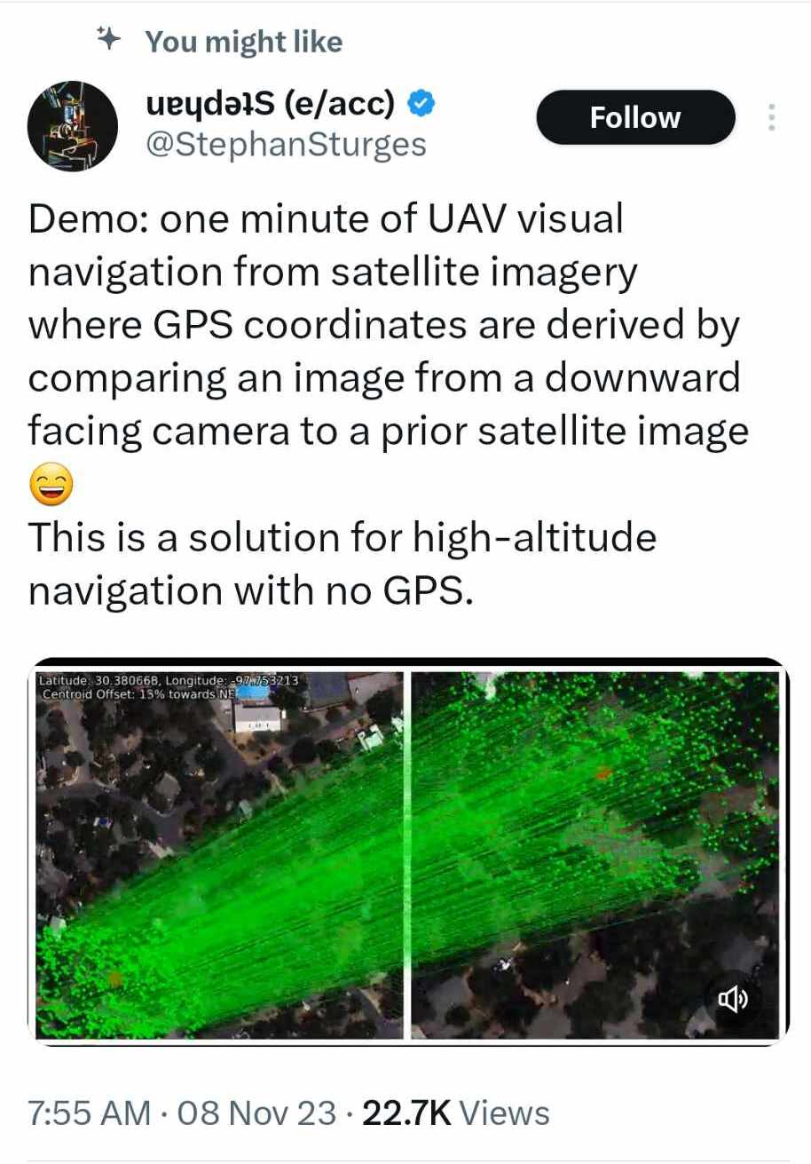
The author of the above tweet employs a reference database of images. It would be interesting to eliminate the need for a raw dataset. Whereas the author employs Visual Place Recognition, here I employ pose estimation techniques. Thus I do not seek to estimate predict place labels, but rather geolocated place coordinates for the camera, as well as the camera’s orientation.
Thus, this works seeks to develop a neural network which maps a terrain image from the agent’s downward-facing camera, to a 6-DOF (position/rotation) representation of the agent in 3-space.
Background
The goal-statement - relating a camera image to a location and orientation in the world - has been deeply studied in computer vision and rendering
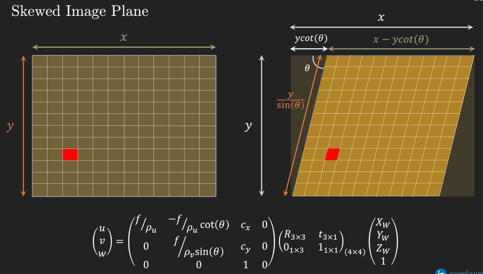
Formally
- The image-formation problem is modeled as a camera forming an image of the world using a planar sensor.
- World coordinates refer to 3-space coordinates in the Earth or world reference frame.
- Image coordinates refer to 2-space planar coordinates in the camera image plane.
- Pixel coordinates refer to 2-space coordinates in the final image output from the image sensor, taking into account any translation or skew of pixel coordinates with respect to the image coordinates.
The mapping from world coordinates to pixel coordinates is framed as two composed transformations, described as sets of parameters
- Extrinsic camera parameters - the transformation from world coordinates to image coordinates (affected by factors “extrinsic” to the camera internals, i.e. position and orientation.)
- Intrinsic camera parameters - the transformation from image coordinates to pixel coordinates (affected by factors “intrinsic” to the camera’s design.)
And so broadly speaking, this work strives to design a neural network that can map from an image (taken by the agent’s downward-facing camera) to camera parameters of the agent’s camera. With camera parameters in hand, geolocation parameters automatically drop out from extracting extrinsic translation parameters.
To simplify the task, assume that camera intrinsic characteristics are consistent from image to image, and thus could easily be calibrated out in any application use-case. Therefore, this work focuses on inferring extrinsic camera parameters from an image. We assume that pixels map directly into image space.
The structure of extrinsic camera parameters is as follows
where \(\mathbf{R}_{3 \times 3} \in \mathbb{R^{3 \times 3}}\) is rotation matrix representing the rotation from the world reference frame to the camera reference frame, and \(\mathbf{t}_{3 \times 1} \in \mathbb{R^{3 \times 1}}\) represents a translation vector from the world origin to the image/camera origin.
Then the image coordinates (a.k.a. camera coordinates) \(P_c\) of a world point \(P_w\) can be computed as
Proposed solution
Image-to-extrinsics encoder architecture
The goal of this work, is to train a neural network which maps an image drawn from \(R^{3 \times S \times S}\) (where \(S\) is pixel side-length of an image matrix) to a pair of camera extrinsic parameters \(R_{3 \times 3}\) and \(t_{3 \times 1}\):
\[\mathbb{R^{3 \times S \times S}} \rightarrow \mathbb{R^{3 \times 3}} \times \mathbb{R^3}\]The proposed solution is a CNN-based encoder which maps the image into a length-12 vector (the flattened extrinsic parameters); a hypothetical architecture sketch is shown below:

Data sources for offline training
Online sources
Training and evaluation
The scope of the model’s evaluation is, that it will be trained to recognize aerial views of some constrained area i.e. Atlantic City New Jersey; this constrained area will be referred to as the “area of interest.”
Data pipeline
The input to the data pipeline is a single aerial image of the area of interest. The output of the pipeline is a data loader which generates augmented images.
The image of the area of interest is \(\mathbb{R^{3 \times T \times T}}\) where \(T\) is the image side-length in pixels.
Camera images will be of the form \(\mathbb{R^{3 \times S \times S}}\) where \(S\) is the image side-length in pixels, which may differ from \(T\).
- Generate an image from the agent camera’s vantage-point
- Convert the area-of-interest image tensor (\(\mathbb{R^{3 \times T \times T}}\)) to a matrix of homogenous world coordinates (\(\mathbb{R^{pixels \times 4}}\)) and an associated matrix of RGB values for each point (\(\mathbb{R^{pixels \times 3}}\))
- For simplicity, assume that all features in the image have an altitutde of zero
- Thus, all of the pixel world coordinates will lie in a plane
- Generate random extrinsic camera parameters \(R_{3 \times 3}\) and \(t_{3 \times 1}\)
- Transform the world coordinates into image coordinates (\(\mathbb{R^{pixels \times 3}}\)) (note, this does not affect the RGB matrix)
- Note - this implicitly accomplishes the commonly-used image augmentations such as shrink/expand, crop, rotate, skew
- Convert the area-of-interest image tensor (\(\mathbb{R^{3 \times T \times T}}\)) to a matrix of homogenous world coordinates (\(\mathbb{R^{pixels \times 4}}\)) and an associated matrix of RGB values for each point (\(\mathbb{R^{pixels \times 3}}\))
- Additional data augmentation - to prevent overfitting
- Added noise
- Color/brightness adjustment
- TBD
- Convert the image coordinates and the RGB matrix into a camera image tensor (\(\mathbb{R^{3 \times S \times S}}\))
Each element of a batch from this dataloader, will be a tuple of (extrinsic parameters,camera image).
Training
- For each epoch, and each mini-batch…
- unpack batch elements into camera images and ground-truth extrinsic parameters
- Apply the encoder to the camera images
- Loss: MSE between encoder estimates of extrinsic parameters, and the ground-truth values
Hyperparameters
- Architecture
- Encoder architecture - CNN vs MLP vs ViT(?) vs …, number of layers, …
- Output normalizations
- Nonlinearities - ReLU, tanh, …
- Learning-rate
- Optimizer - ADAM, etc.
- Regularizations - dropout, L1, L2, …
Evaluation
For a single epoch, measure the total MSE loss of the model’s extrinsic parameter estimates relative to the ground-truth.
Feasibility
Note that I am concurrently taking 6.s980 “Machine learning for inverse graphics” so I already have background in working with camera parameters, which should help me to complete this project on time.
Implementation
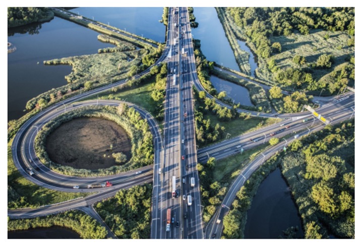
Source image
DOF estimation was applied to a 2D aerial image
Dataloader
A dataloader was created which generates (1) generates a random extrinsic camera matrix as described above, in order to generate (2) visualization of the above source image from the perspective of the random camera matrix.
More specifically, the dataloader generates Euler Angles in radians associated with with the camera matrix rotation, as well as a 3D offset representing the camera’s position.
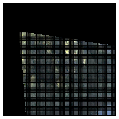
You will notice that the images suffer from an artifact whereby the pixels are not adjacent to each other but rather have black space between them; a production implementation of this solution would require interpolation between pixels in order to produce a continuous image.
An example of a single generated image is shown below; it is the original image, above, viewed from the perspective of a random camera matrix:
A batch of generated images is shown below:
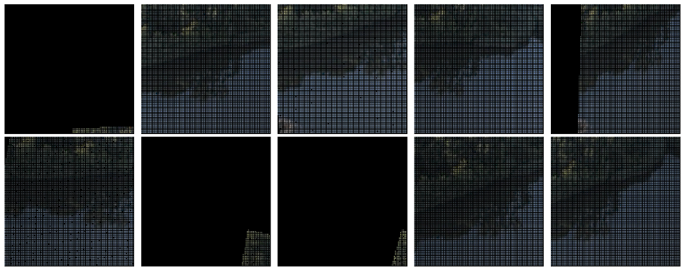
Again, you can see that owing to a lack of interpolation, the pixels are spread out, with black space between them.
DNN architecture
The DNN architecture is an MLP with 6 hidden layers of width 512, 256 and 128.
The input is a 224x224 image with 3 color channels representing the view of the source image from an orientation determined by the (unknown) camera extrinsic parameters.
The architecture outputs 6 logit values values corresponding to predictions of 3 Euler angles and 3 positional offsets for the camera extrinsic matrix.
For this project, I experimented with the sinusoidal activation functions described in the SIREN
One question which might arise is, if the DNN outputs logits, how do I account for the difference in statistical characteristics between the three Euler Angle outputs and the three translation vector outputs? I employed scikitlearn StandardScalers at both the input and the output in order to normalize image pixels and extrinsic camera matrix parameters, respectively. The use of normalization at the input is standard. The use of normalization at the output allows each dimension of the 6-logit output to learn a zero-mean, unit-variance distribution: the output StandardScaler converts from zero-mean, unit-variance to the estimated actual mean and variance of the target distribution. The way the output StandardScaler is computed is as follows: a batch of random data is sampled from the dataloader; mean and variance are computed; then a StandardScaler is designed such that its inverse maps from the computed mean and variance of the target extrinsics, to zero mean/unit-variance. Thus, run forward, the output StandardScaler will map from unit gaussian to the computed mean and variance.
Training setup
I train for 80 epochs with an Adam optimizer and a learning rate of 0.00001.
MSE loss is employed for training and evaluation. The extrinsic parameters predicted by the DNN are compared against the target (correct) extrinsic parameters which the dataloader used to generate the camera image of the scene. Recall from the previous section that, owing to the output StandardScaler, the DNN outputs 6 roughly zero-mean/unit-variance predicted camera extrinsic parameters. I chose to evaluate loss relative to these zero-mean/unit-variance predictions, prior to the output StandardScaler; the rationale being that I wanted each extrsinsic parameter to have equal weighting in the MSE loss computation, and not be biased by the mean/variance of the particular parameter. Thus, I use the output StandardScaler in inverse mode to normalize the target values to zero-mean/unit-variance. MSE loss is then computed between the DNN output logits, and these normalized target values.
A side-effect of computing MSE against normalized values, is that it is effectively a relative measure: MSE tells me how large the variance in the error between predictions and target is, relative to the unit-variance of the normalized target values. Thus I expect that an MSE much less than one is a good heuristic for the quality of the estimate.
Training results
The plot below shows that the DNN architecture was able to converge on low-MSE predictions of the extrinsic camera matrix:
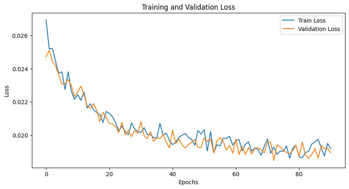
Note that the train and test curves overlap almost perfectly; this is because all datapoints generated by the dataloader are random, so in fact the model is constantly being trained on fresh data, and the resampling is really unnecessary.
Since the final MSE is relatively small (0.020), and since (as described in the previous section) the MSE is effectively a relative measure of error, I believe the DNN is learning a relatively good estimate of camera extrinsics.
Conclusion
Based on the low MSE attained during training, I believe I successfully trained a DNN to roughly estimate camera extrinsics from orientation-dependent camera views.
There are many improvements which would be necessary in order to deploy this in production.
For example, it would be better to use more detailed satellite imagery, preferably with stereoscopic views that effectively provide 3D information. Without having 3D information about the scene, it is hard to train the model to recognize how the scene will look from different angles. In my work, I used a 2D image and essentially assumed that the height of the geographic features in the image was negligible, such that I could approximate the 3D point-cloud as lying within a 2D plane. With stereoscopic satellite data, it could be possible to construct a truly 3D point-cloud, on which basis I could synthesize more accurate camera views during the training process.
Also, as discussed in the Implementation section, it would likely be necessary to implement interpolation between the pixels when generating simulated camera views. Otherwise, the camera views during training would look nothing like what the camera would see in the real world.