Optimizations of Transformers for Small-scale Performance
CNNs generally outperform ViTs in scenarios with limited training data. However, the narrative switches when the available training data is extensive. To bridge this gap and improve upon existing ViT methods, we explore how we can leverage recent progress in the transformer block and exploit the known structure of pre-trained ViTs.

Figure 1: Attention Maps of a Vision Transformer (DINO). Source: https://github.com/sayakpaul/probing-vits .
Transformers: Great but fall short
Basic Background
Transformers have well-earned their place in deep learning. Since the architecture’s introduction in
Originally designed for NLP, the transformer architecture has been robust in other domains and tasks. For example, it has been translated, with success, to de-novo protein design
Vision: The Problem
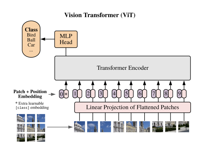
The Vision Transformer (ViT)
Since its introduction, the ViT and associated variants have demonstrated remarkable benchmarks in image classification
Despite the complementary nature of these architectures, they break the fidelity of the transformer and make for difficult analysis. Therefore, there exists a gap in the traditional transformer architecture to perform in small-data regimes, particularly in vision. Motivated by this shortcoming, we aim to investigate and improve the current ViT paradigm to narrow the gap between CNNs and ViTs on small-data. In particular, we examine novel initialization schemes, removal of component parts in our transformer block, and new-learnable parameters which can lead to better performance, image throughput, and stable training on small-scale datasets.
Transformer Block
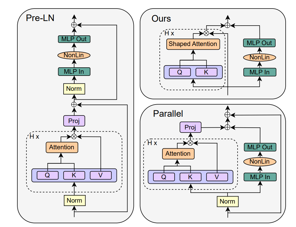
To serve as a basis of comparison, we will examine the stanford transformer block seen in Figure 3. The block is identical to
Before we delve into these advances and their implications, consider the following transformer block information flow:
\[\displaylines{ \text{Attention} = \text{A}(X) = \text{Softmax}\Biggl(\frac{XW_{Q}W_{K}^{T}X^{T}}{\sqrt{k}}\Biggl) \\ \\ \text{A}(X) \in \mathbb{R}^{T\times T}}\]which is shortly followed by:
\[\displaylines{ \text{S}(X) = \text{A}(X)W_{V}W_{O} \\ \\ \text{S}(X) \in \mathbb{R}^{T\times d} }\]and:
\[\text{Output} = \text{MLP}(\text{S}(X))= \text{Linear}(\text{GELU}(\text{Linear}(\text{S}(X))))\]where:
- Embedded input sequence: \(X \in \mathbb{R}^{T \times d}\)
- Linear queury and key layers: \(W_{Q},W_{K} \in \mathbb{R}^{d \times k}\)
- Linear value and projection layers: \(W_{V}, W_{O} \in \mathbb{R}^{d \times d}\)
- MLP Linear layers: \(\text{Linear} \in \mathbb{R}^{d \times d}\)
- \(T =\) # of tokens, \(d =\) embedding dimension, \(k = \frac{d}{H}\), \(H =\) # of attention heads
The flow of information mirrors the transformer block in Figure 3. Readers unfamiliar with transformer intricacies such as MHA and MLPs are encouraged to read
Recently, there have been many proposals on how the transformer block can be further modified to increase data throughput and eliminate “redundant” or “useless” parts that do not have any significant contribute to the tranformer’s modeling capabilities. For example,

The overaching theme of
where \(\alpha\) and \(\beta\) are learnable scalars and intialized to \(1\) and \(0\), respectively, and \(\text{I} \in \mathbb{R}^{T \times T}\) is the identity matrix. This modification intiailizes the self-attention matrix providing a pathway towards training stability. They further entertained a more complicated scheme with a third parameter, but we only consider the two parameter version for simplicity. By this iterative removal and recovery process, the authors converged towards the final transformer block seen in Figure 4. The most shocking aspect of this proposed block is the removal of the \(W_{V}\) and \(W_O\) layers. They arrived to this justification by initialializing \(W_{V}\) and \(W_{O}\) to the identity with separate, learnable scalars and training a model. Over the course of training, the scalar ratios converged towards zero
import torch
import torch.nn as nn

class ShapedAttention(nn.Module):
    def __init__(self, width: int, n_hidden: int, num_heads: int):
        super().__init__()
        # Determining if hidden dimension of attention layer is divisible by number of heads
        assert width % num_heads == 0, "Width and number of heads are not divisble."

        # Setting vars
        self.head_dim   = n_hidden // num_heads
        self.num_heads  = num_heads
        # Creating Linear Layers
        self.W_K = nn.Linear(width, self.head_dim)
        self.W_Q = nn.Linear(width, self.head_dim)
        # Learnable Scalars: alpha_init and beta_init are up to user
        self.alpha = nn.Parameter(alpha_init)
        self.beta = nn.Parameter(beta_init)
        # Softmax
        self.softmax = nn.Softmax(dim = -1)

    def forward(self, x: torch.Tensor) -> torch.Tensor:
        # Input:
        # x: shape (B x T x dim)
        # Outputs:
        # attn_output: shape (B x T x width)
        attn_output = None
        # Compute keys and queries
        k = self.W_K(x)
        q = self.W_Q(x)
        # Scaled dot-product
        attn_scores = torch.bmm(q, k.transpose(1,2)) / (self.head_dim**-0.5)
        attn_scores = self.softmax(attn_scores)
        # Shaped attention
        B, T, _ = x.shape
        output = self.alpha*torch.eye(T, device = x.device) + self.beta * attn_scores

        return output
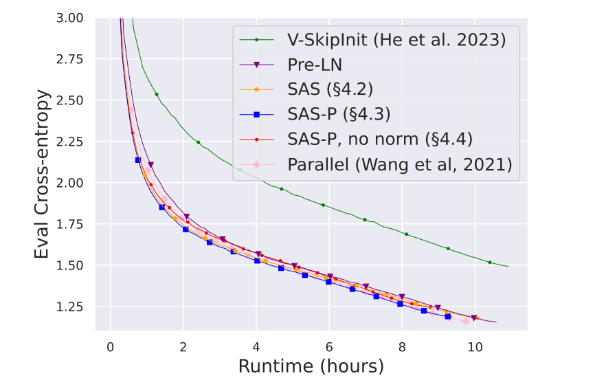
The performance of the final transformer block (referred to as SAS-P) demonstrated powerful results. In the Figure, the simplified transformer matches the standard block in cross-entropy loss even when taken through a long runtime. Additionally, Figure 6 in

Translation to Vision: Experimentation and Analysis
The results shown in
Vanilla vs. Simplified Comparison
For evaluation, we compare the simplified transformer to a vanilla ViT. The vanilla ViT’s transformer block is identical to the formulation presented earlier. We use Conv2D patch embedding with a random initial positional embedding. For the simplified setup, we initialize \(\alpha = \beta = 0.5\) and do not use a centering matrix – although it has been shown to improve ViT performance
| Table 1. Experiment 1: ViT Model Settings | |
|---|---|
| # of channels | 3 |
| Image size | 32 |
| Patch size | 4 |
| Width | 96 |
| # of heads | 4 |
| # of layers | 8 |
| Table 2. Experiment 2: Results | Vanilla | Simplified | \(\Delta\) |
|---|---|---|---|
| Parameters | 358186 | 209210 | -41.59% |
| Avg. epoch time (s) | 12.954 | 11.305 | -12.73% |
Experiment 1 showed the training evaluation trajectory is nearly identicable between the two models although the simplified outperforms by small margin. Although the subtle difference, it is noteworthy to mention the simplified version achieved mirroring performance with less parameters and higher image throughput. The similarity of the curves hints the removal of the skip connections, layer normalizations, and value/projection layers were merited, begging the question whether these components held our modeling power back.
This experimentation shows the similar nature of each model, but does not translate well to wider modern neural networks. In Experiment 2, we expanded to \(\text{width} = 128\) to determine if there is any emergent behaviour as the network becomes wider. We replicate everything in Experiment 1 and solely modify the width. The settings are restated in Table 3. The results for Experiment 2 can be seen in Figure 7 and Table 4 below.
| Table 3 | Experiment 2: ViT Model Settings |
|---|---|
| # of channels | 3 |
| Image size | 32 |
| Patch size | 4 |
| Width | 128 |
| # of heads | 4 |
| # of layers | 8 |
| Table 4. Experiment 2: Results | Vanilla | Simplified | \(\Delta\) |
|---|---|---|---|
| Parameters | 629130 | 364954 | -41.99% |
| Avg. epoch time (s) | 13.093 | 11.735 | -10.37% |
The narrative is different for Experiment 2. The simplified version outperforms the vanilla version by a considerable margin. An adequate explanation for this discrepancy in vision tasks merits further exploration. However, considering the proposed unnecessary nature of the value and projection matrices, we can hypothesize they interfere with the modeling capability as more parameters are introduced.
Due to the sheer difference in outcomes between the models, we question how the models are attending towards various inputs to gain a better understanding of what is happening under the hood. To probe this curiosity, we trained the models with identical setting in Experiment 2, but modified the \(\text{depth} = \text{layers} = 12\). This model setup will be covered in more detail in future paragraphs. We inputted CIFAR-10 to each model and visualized a side-by-side comparison of attention maps for five input images. An interactive figure is seen Figure 8.
There is a noticeable contrast in the attention maps. For the simplified model, the attention maps seem to place weight in a deliberation manner, localizing the attention towards prominent features in the input image. On the other hand, the vanilla model is choatic in its attention allocation. It is noteworthy that the vanilla model does place attention towards areas of interest, but also attends towards irrelevant information perhaps compromising its judgement at the time of classification. It can thus be reasoned the simplified model can better decipher which features are relevant demonstrating, even in low data regimes, the representational quality is increased.
While we have so far investigated width, it will be informative to understand how depth impacts the performance of the simplified version. In
| Table 5. Experiment 3: Results | Vanilla | Simplified | \(\Delta\) |
|---|---|---|---|
| Parameters | 927370 | 531106 | -42.72% |
| Avg. epoch time (s) | 17.527 | 15.723 | -10.29% |
Again, the simplified model outperforms the vanilla model by a large margin. Although we have focused on performance in the past, we discern an interesting trend when we scaled the depth: the simplified version seemed to be more consistent from run-to-run (recall \(\text{runs} = 5\)). This leads us to believe that as we continue to scale the depth, the simplified version will be more stable. Future experimentation will be necessary to corroborate this claim.
Initialization Schemes
We have seen the impact simplification can have on the performance of the transformer performance and self-attention. However, the used initializatons of \(\alpha\) and \(\beta\) in Experiments 1, 2, and 3, was based on equal weighting between the initial attention matrix and the identity matrix. In
This lead us to believe the initializaton scheme could be improved. There has been some work on initializing vanilla ViTs
To give more evidence to this hypothesis, we experimented with the following dynamic initialization scheme:
\[\displaylines{ \alpha_i = \frac{1}{i}, \beta_i = 1 - \frac{1}{i} \\ \text{ where } i \in [1, 2, ..., L] \text{ and } L = \text{# of layers} }\]The results from this initialization scheme compared to the uniform initializations can be seen in Figure 12 The results show that the dynamic scheme outperform the results perhaps indicating the representation quality is connected toward encouraging self-token connection in the lower layers, while allowing for token’s to intermingle in higher layers. We further experiment with the inverse dynamic where we switch the \(\alpha\) and \(\beta\) values. The results in Figure 13 show the dynamic approach is stronger during training then the inverse dynamic approach.

Conclusion and Limitations
Through this blog post we have overviewed the simplification of our known transformer block and novel initialization schemes. We took the problem of small-scale training of ViT’s and looked to address it leveraging such ideas. Through a series of experiments and thoughtful schemes, we generated an informed and sophisticated approach to tackle such a problem. In the end, we generated a method that outperformed a tradtional ViT in small scales. We explored ways of scaling the ViT in width and depth and probed how the new model distributed attention. Our comparisons were intentionally simple and effective in addressing the underlying task and illustrating the models potential. Although the results presented showed promise, extensive validation needs to be performed in the future. It will be interesting to see how this new transformer block and intialization scheme can be further utilized in computer vision. For example, a logical next route to entertain is to compare convergence rates in larger scale ViT on datasets such as ImageNet-21k to see if the modeling advantage persists.
There are a few limitations in this study. For one, only one dataset was used. Using other datasets such as CIFAR-100 or SVHN would provide more insight into this methodology. Secondly, there is a need for more comprehensive evaluation and ablation studies to determine the true nature of the simplified transformer and initialization schemes. Third, a comparison to a smaller scale CNNs is needed to gauge where this method comparatively sits in modeling power.

