VGAE Clustering of the Fruit Fly Connectome

An exploration of how learned Variational Graph Auto-Encoder (VGAE) embeddings compare to Spectral Embeddings to determine the function of neurons in the fruit fly brain.

Motivation

The fruit fly connectome.

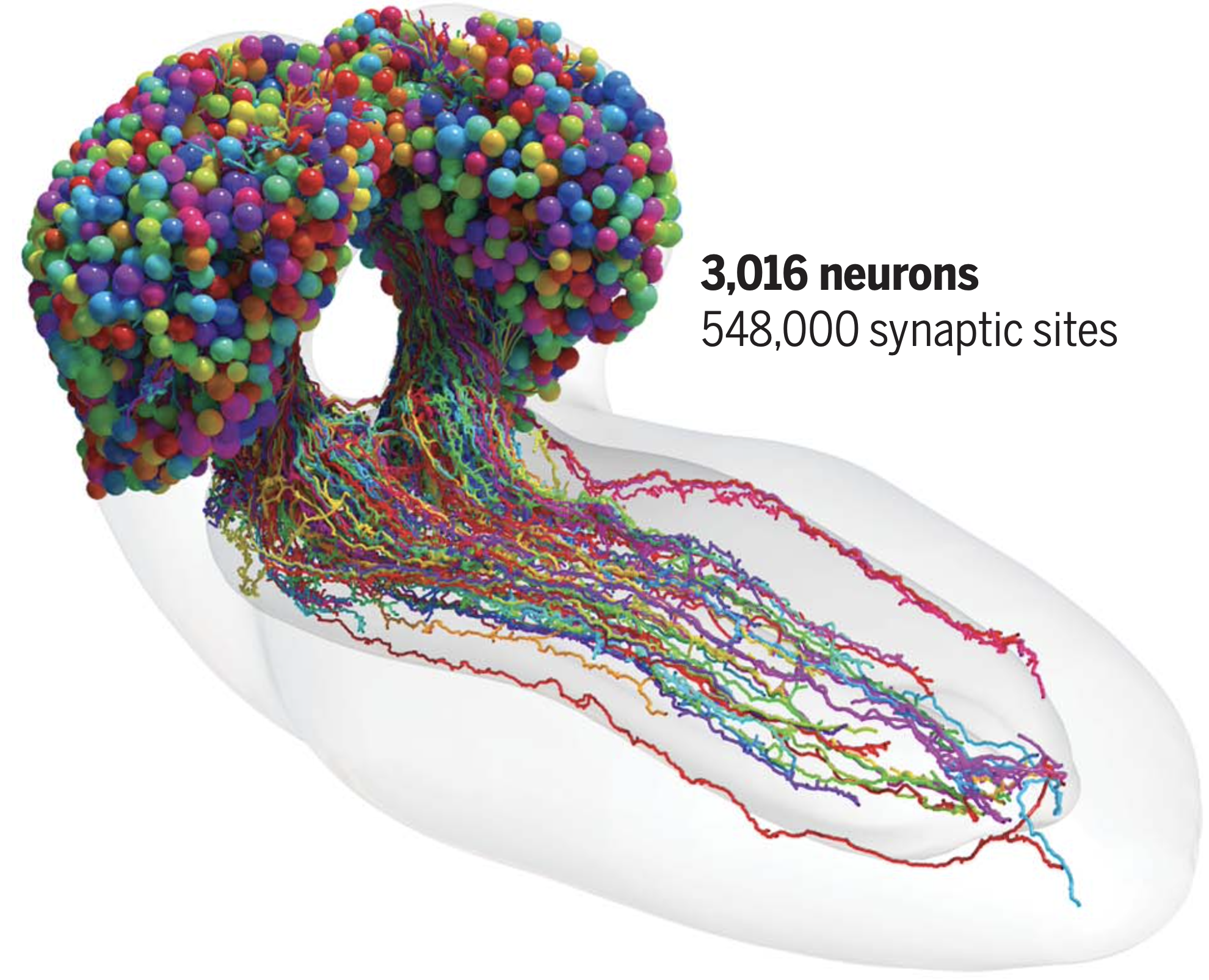
Everything you’ve ever learned, every memory you have, and every behavior that defines you is stored somewhere in the neurons and synapses of your big, beautiful brain. The emerging field of connectomics seeks to build connectomes–or neuron graphs–that map the connections between all neurons in the brains of increasingly complex animals, with the goal of leveraging graph structure to gain insights into the functions of specific neurons, and eventually the behaviors that emerge from their interactions. This, as you can imagine, is quite a difficult task, but progress over the last few years has been promising.

Now, you might be asking yourself, can you really predict the functions of neurons based on their neighbors in the connectome? A paper published by Yan et al. in 2017 asked this same question, searching for an answer in a roundworm (C. elegans) connectome. In their investigation, they discovered a neuron whose behavior had not been previously characterized, which they hypothesized was necessary for locomotion. They tested this hypothesis by ablating the neuron on a living C. elegans, and to the dismay of that poor roundworm, found that it was indeed necessary.

Although impressive, the C. elegans connectome has only ~300 neurons, compared with the ~100,000,000,000 in the human brain; however, this year (2023):

1. A paper by Winding et al. has published the entire connectome of a fruit fly larvae, identifying 3016 neurons and their 548,000 synapses.
2. Google Research has announced an effort to map a mouse brain (~100,000,000 neurons)

This is exciting because the fruit fly dataset presents an opportunity to identify more nuanced functions of neurons that may be present in more complex species like mice, but not in simpler species like the roundworm. This creates the requirement for algorithms that are sufficiently expressive and able to disentangle the similarities between neurons that appear different, but are functionally similar.

Furthermore, current efforts to map connectomes of increasingly complex animals makes it desirable to have algorithms that are able to scale and handle that additional complexity, with the hopes of one day discovering the algorithms that give rise to consciousness.

Background

Can we learn about human brains by studying connectomes of simpler organisms?

The primate brain exhibits a surprising degree of specialization, particularly for social objects. For instance, neurons in the face fusiform area (FFA) in the IT cortex appear to fire only in response to faces. Furthermore, individuals with lesions in or brain damage to this area lose their ability to recognize faces . In fact, there is even evidence of rudimentary face perception even in newborn infants with limited access to visual “training data,” who preferentially look at photos of faces, and other face-like arrangements, like inverted triangles (two vertices being the eyes and the third the mouth) . While there may not exist a grandmother cell that can recognize your grandmother, there certainly seems to be at least some engineered specialization in the brain. Cognitive scientists theorize that there is a set of core systems for representing object, actions, number, space, and conspecifics (other people!), together constituting what we might call “common sense,” which may help determine the blueprint of the human brain down to the genetic level . Notably, facial recognition exhibits substantial genetic heritability (over 60%!) and appears to be uncorrelated with general intelligence . We might imagine that there are a set of capabilities, including social cognition, that were so critical for human behavior that our brains evolved over hundreds of thousands of years to “hard code” certain structures, like the FFA, to help scaffold them. After all, another person’s face is an important signal for processes like mate selection, friendship formation, and theory of mind. The human brain and the cognitive processes it supports are evolutionary products. And even more importantly, the brain seems to be specialized in some ways, but behave flexibly in others. Through the scientific process, how good of an understanding can we reach about the complex organ sitting between our ears? To what degree are the neuronal assemblages in our brain specialized? How do the communications amongst these neurons grant us our incredible cognitive capabilities?

In 1982, neuroscientist David Marr proposed three levels of analyses to study complex systems like the human mind: the computational level (what task is the system designed to solve?), the algorithmic level (how does the system solve it?), and the implementation level (where and how is the algorithm implemented in the system hardware?) . At one end of the spectrum, we might think about characterizing the computational capabilities of human cognition, like object recognition. On the other end, we might be interested in how object recognition is implemented in the brain itself, in all of its fleshy glory–how an incoming visual signal is processed by composites of receptive fields in the retina (biological “Gabor filters”) and fed to neurons in the primary and secondary visual areas of the cerebral cortex, for instance . In recent years, scientists have developed an interest in understanding the implementation level at an extremely high resolution by charting the connectome–the comprehensive map of all neural connections in the brain. However, if the grandmother cell is too simplistic of a model for knowledge representation in the human brain, then indeed the human connectome may offer an overly complex view. It seems easy to get lost in the wilderness of its approximately 100 trillion neurons and the nearly quadrillion synapses which connect them ! How can we begin to approach this overwhelming terra incognita?

We might consider instead studying the connectome of a much simpler model organism, like the transparent 1mm-long nematode Caenorhabditis elegans, with whom we share an estimated 20-71% of our genes with . Or, maybe even the fruit fly Drosophila melanogaster, 60% of whose genes can also be found in the human genome (Max Planck). Even the study of such model organisms necessitates adding structure to complex, often unlabeled, relational data. And while the fruit fly brain is orders of magnitude less complex than our own, there are still over 3,000 neurons and half a million synapses to explore (Winding et al., 2023). Luckily, mankind’s toolkit for studying graph-like data is well-equipped.

Unsupervised graph representation learning

The problem of subdividing neurons in a connectome into types based on their synaptic connectivity is a problem of unsupervised graph representation learning, which seeks to find a low-dimensional embedding of nodes in a graph such that similar neurons are close together in the embedding space.

A common way to identify functional clusters of neurons is through the lens of homophily, meaning that neurons serve the same function if they are within the same densely connected cluster in the connectome; however, this fails to capture the likely case that neurons with similar low-level functions span across many regions of the brain.

Instead, a better approach might be to cluster neurons based on their structural equivalence, such that groups of neurons with similar subgraph structures are embedded similarly, regardless of their absolute location in the connectome. This is the approach taken by Winding et al., who “used graph spectral embedding to hierarchically cluster neurons based on synaptic connectivity into 93 neuron types”. They found that even though they used only information about the graph structure to predict functions, neurons in the same clusters ended up sharing other similarities, including morphology and known function in some cases.

Spectral embedding is a popular and general machine learning approach that uses spectral decomposition to perform a nonlinear dimensionality reduction of a graph dataset, and works well in practice. Deep learning, however, appears to be particularly well suited to identifying better representations in the field of biology (e.g., AlphaFold2), and deep learning methods do appear to be capable of creating embeddings that more effectively preserve the topology of nodes in graphs.

Learned VGAE graph embedding for Cora citation network dataset.

Thus, it stands to reason that deep learning might offer more insights into the functions of neurons in the fruit fly connectome, or at the very least, that exploring the differences between the spectral embedding found by Winding et al. and the embeddings discovered by deep learning methods might provide intuition as to how the methods differ on real datasets.

In this project, we explore the differences between functional neuron clusters in the fruit fly connectome identified via spectral embedding by Winding et al. and deep learning. Specifically, we are interested in exploring how spectral embedding clusters differ from embeddings learned by Variational Graph Auto-Encooders (GVAE), which are a more recent architecture proposed by one of the co-authors of the Variational Auto-Encoders (VAE) paper, Max Welling. GVAEs are an interesting intersection of graph neural networks (GNNs) and VAEs, both of which we explored in class, and comparing this technique to spectral embedding is relevant because of our previous discussions of spectral decomposition in class with respect to network scalability and RNN weights.

We hypothesize that a deep learning technique would be better suited to learning graph embeddings of connectomes because they are able to incorporate additional information about neurons (such as the neurotransmitters released at synapses between neurons) and are able to learn a nonlinear embedding space that more accurately represents the topological structure of that particular connectome, learning to weight the connections between some neurons above others.

Before we can discuss the experiments, however, we first provide more detail for Spectral Embedding and Graph Variational Autoencoders and compare the two methods.

Methods

Spectral Embedding

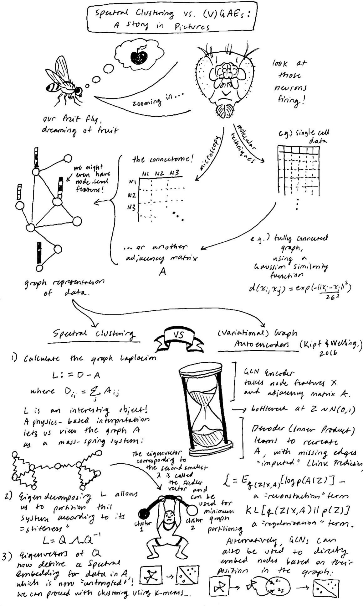
One classical approach for understanding graph-like data comes from a class of spectral methods which use pairwise distance measures between data points to embed and cluster data. Spectral methods offer two obvious advantages when compared to other machine learning approaches. One, we can straightforwardly perform clustering for datasets which are inherently relational, like the connectome, where it is not immediately clear how a method like k-means can be used when we only have access to the relationships between data points (the “edges”) and not the node-level features themselves. Two, spectral methods are nonlinear, and don’t rely on measures like squared Euclidean distance, which can be misleading for data which are tangled in high dimensions, but which exhibit a lower intrinsic dimensionality.

So, how does spectral embedding work, exactly? In short, an adjacency matrix is first calculated from the original dataset, which is then used to compute the graph Laplacian. Next, a normalized graph Laplacian is then eigen-decomposed and generates a lower dimensional embedding space on which simpler linear clustering algorithms, like k-means, can be used to identify untangled clusters of the original data.

This class of methods makes no assumptions about the data (including cluster shape) and can be adjusted to be less noise sensitive–for example, by performing a t-step random walk across the affinity matrix for the data, as in diffusion mapping . An added benefit is that under the hood, spectral embedding can be performed by a series of linear algebra calculations, making it extremely time-efficient. However, as with many unsupervised learning methods, clustering based on spectral embeddings is difficult to scale–in our case, due to the eigen-decomposition step of the graph Laplacian.

Variational Graph Autoencoders

Although Spectral Embedding is still very popular, in recent years, more attention has been paid to the burgeoning field of geometric deep learning, a set of ideas which aim to to solve prediction or embedding tasks by taking into account the relational structure between data points. One example is the variational graph auto-encoder (VGAE), which learns to embed a complex object like a network into a low-dimensional, well-behaved latent space. Kipf and Welling (2016) propose an encoder using a two-layer graph convolutional network, which performs convolutions across local subgraphs of the input network data (not unlike convolution on images, where the graph is a grid!). The graph is projected onto a low dimensional space distributed according to the standard normal through the optimization of a variational lower bound loss, and then upsampled using an inner product between latent variables. They show that this method achieves competitive results on a link prediction task when compared to other methods like spectral clustering and DeepWalk, a random walk-based representation learning algorithm.

On the other hand, some have discovered that spectral embedding leads to more clear separability in low dimensional representation spaces for text data compared to GNN approaches like node2vec, which reportedly achieve state-of-the-art (sota) scores for multilabel classification and link prediction in other datasets . In addition, it appears that simple modifications like performing an error correlation correction on the training data and smoothing predictions on the test data for GNN-free architectures lead to sota-comparable performances . There are even concerns that the performance of geometric deep learning approaches are inflated, particularly in tasks like multi-label node classification, due to the assumption that the number of labels for test data are known to researchers .

Thus, it remains unclear in what circumstances relatively novel geometric deep learning approaches do better compared to established and widely-explored methods like spectral learning, and particularly for novel data like the connectome. In this work, we attempt to gain deeper insights into which method is moroe well-suited to the task of connectome modeling, with the hope of learning about which method should be implemented in future connectomes, such as that of the mouse and eventually the human.

Spectral Clustering (von Luxburg, 2007; Park, Jeon, & Pedryc, 2014) vs (V)GAEs (Kipf & Welling, 2016): A Story in Pictures

Experiments

Now that we have a good idea of how these methods compare to each other in terms of implementation, we explore them from an experimental perspective. Through our experiments, we try to quantitatively and qualitatively address the question of how connectome clusters learned by GVAE compare to the spectral clusters found in the paper. To answer this question, we make use of the fruit fly connectome adjacency matrix provided by Winding et al. as our primary dataset with the hope of answering this question for our readers.

Experiment 1: Link Prediction

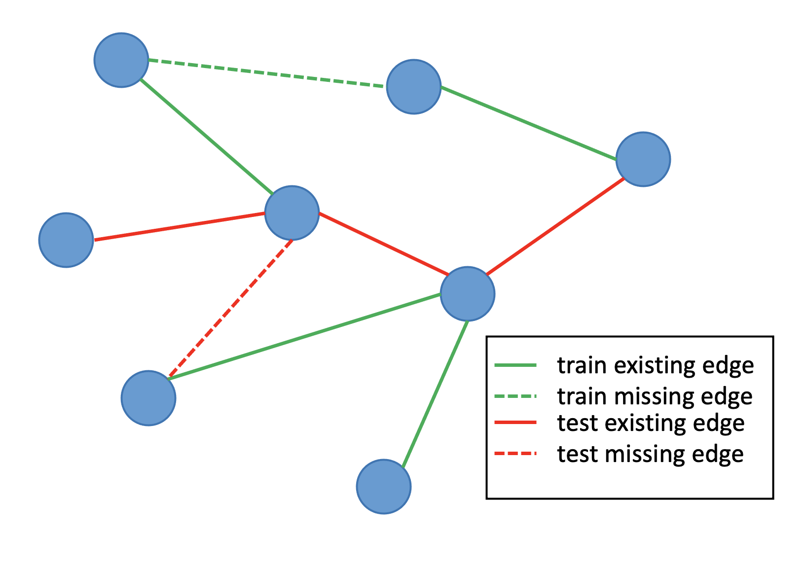
One common way to compare unsupervised graph representation learning algorithms is through a link prediction task, where a model is trained on a subset of the edges of a graph, and then must correctly predict the existence (or non-existence) of edges provided in a test set. If the model has learned a good, compressed representation of the underlying graph data structure, then it will be able to accurately predict both where missing test edges belong, and where they do not.

A link prediction task. Green lines correspond to the training data, which contains samples of positive samples of edges that are present in the graph, and negative samples of edges that are not present in the graph. The test set in red corresponds to the remainder of positive and negative samples in the graph.

We evaluate the models by computing the area under curve (AUC) of the ROC curve, which plots the true positive rate against the false positive rate. A completely random classifier that does not learn anything about the underlying graph structure would get an AUC of 0.5, while a perfect classifier would have an area of 1.0.

Another metric we use to evaluate how good the models are is average precision (AP) of the precision-recall curve, which describes the consistency of the model.

In addition to comparing the models with these metrics, we also explore how robust they are to decreasing dimensionalities of the latent space. We hypothesize that if a model is able to maintain high AUC and AP, even at very low-dimensional embedding spaces, then it is likely better at capturing the structure of the connectome and is more likely to be able to scale to larger datasets, like that of the human brain one day.

Running this experiment yields the following curves, where the x-axis shows the dimensionality of the latent space, and the y-axis shows the AUCs and APs of the respective models.

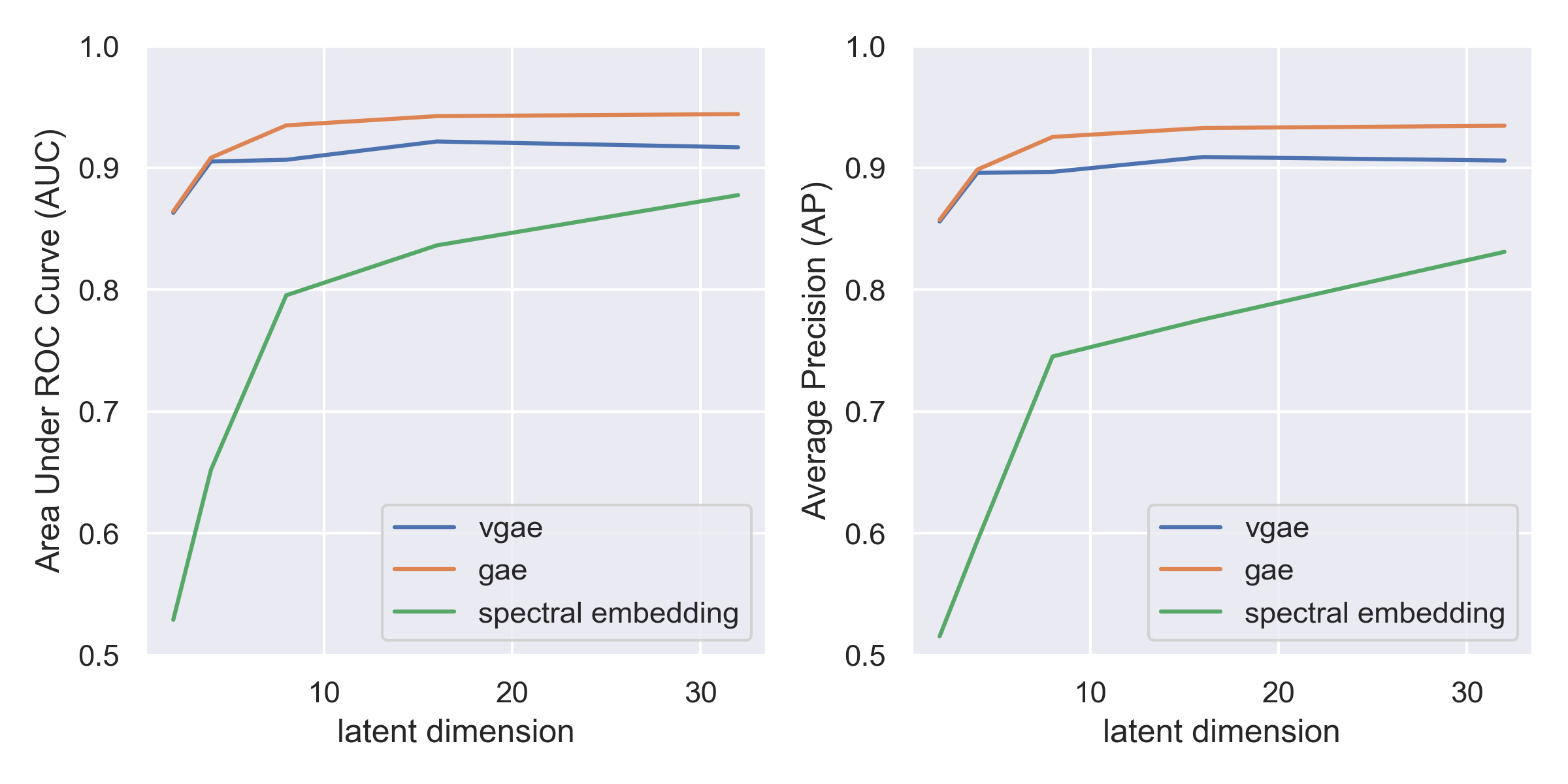
From this experiment, we find that both the Graph Autoencoder (GAE) and Variational Graph Autoencoder (VGAE) perform better than Spectral Embedding methods in terms of AUC and AP, indicating that the models might be better suited to capturing the nuances in the fruit fly connectome. At the dimensionality used for spectral embedding in Winding et al., d=24, we find that the models have comparable performance, but as we reduce the dimensionality of the learned embedding, the spectral embedding method quickly breaks down and loses its ability to capture significant features in the data, with an AUC of 0.52 at a dimensionality of 2. Since a score of 0.5 corresponds to a random model, this means that the spectral embedding method is no longer able to capture any meaningful structure in the data at that dimensionality. Winding et al. gets around this by only using spectral embedding to get a latent space of size 24, and then performing a hierarchical clustering algorithm inspired by Gaussian Mixture Models, but the simplicity and robustness of the GAE model seems to show that they may be better suited to modeling the types of functional neurons present in the connectomes of animals.

Experiment 2: GVAE Latent Exploration

Although the link-prediction experiment gives us a quantitative comparison of the models, we also believe it is important to explore the latent embeddings learned by GAE to see how they qualitatively compare with the learned embeddings used in the Winding et al. work. After observing that the GAE was robust to a latent space of size 2, we decided to look specifically at if there were any similarities between the clusters found by the GAE with the 2-d embedding and the level 7 clusters published by Winding et. al. Also, although the GAE showed better overall performance, we decided to specifically explore the Variational GAE because we expect it to have a latent manifold similar to that of the Variational Autoencoders.

To this end, we first trained a Variational GAE with a 2-d latent space on the full fruit fly connectome and extracted the latent embedding of each node in the connectome.

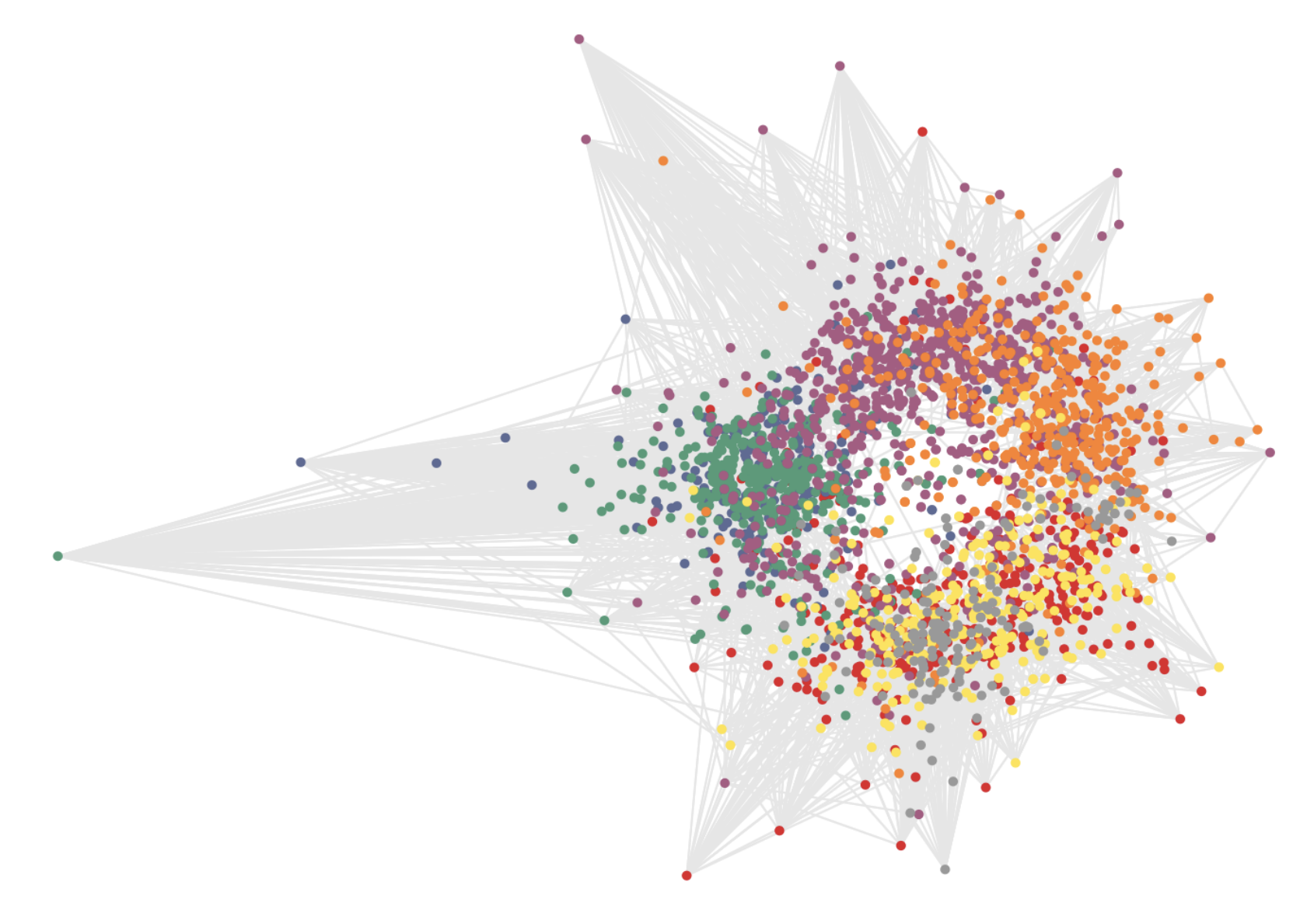
With this latent embedding, we first visualized the latent space using colors corresponding to the 93 clusters identified by Winding et al. Clusters of the same color in the learned GAE latent space mean that the VGAE identified the same cluster that was identified in the Winding et. al. paper and areas where there are many colors within a cluster mean that GAE found a different cluster compared to spectral embedding.

Coloring the GVAE latent space by the found level 7 clusters Winding et al. Black points correspond to neurons that were not assigned a cluster by Winding et al.

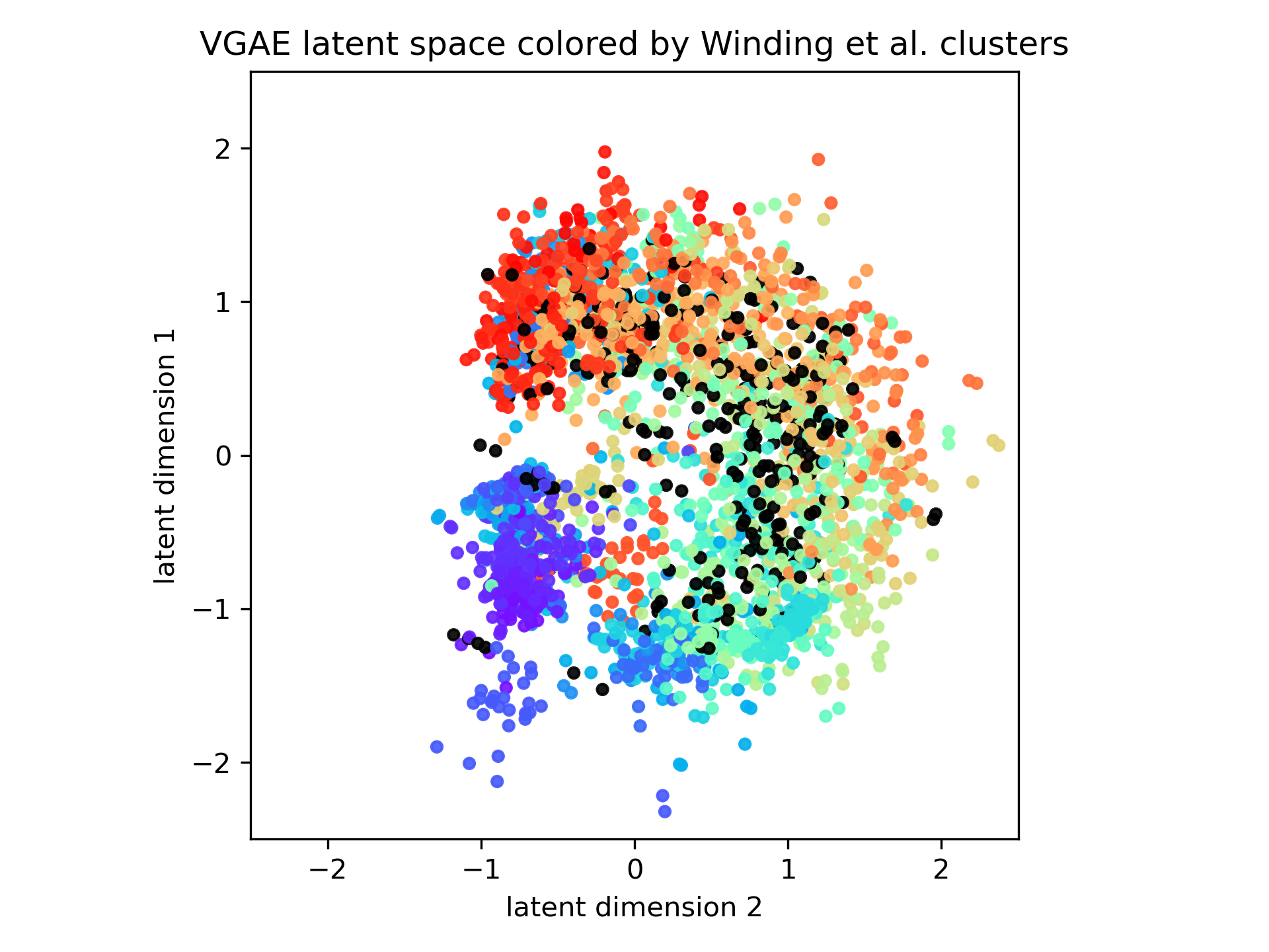
As seen in the figure above, we find that while VGAE projects directly to a 2-d latent space without any additional clustering to reduce the dimensionality, the learned embedding still shares many similarities with the spectral embedding down to a dimensionality of 24 followed by Gaussian Mixture Model hierarchical clustering. Therefore, using VGAE to learn a direct 2-d latent space still captures much of the same information that a more complex machine learning algorithm like spectral embedding is able to.

We further explored the learned latent space by looking at whether the learned embedding had any correlation with the cell types identified in the fruit fly larvae connectome. Since the VGAE only had information about the structure of the graph embedding, clusters of similar colors in this figure mean that the cell type within the cluster shared a lot of common structures, like potentially the same degree or being connected to similar types of up or downstream neurons.

We use the same color palette as the Winding et al. paper so that cell types in the level 7 clusters of the Winding et al. paper can be directly compared to the learned VGAE latent embedding.

Coloring the Winding et al. level 7 clusters (left) and GVAE latent space (right) by cell types. This information was not provided to either algorithm during training, so clusters of the same cell type mean that its type can be inferred from structure only.

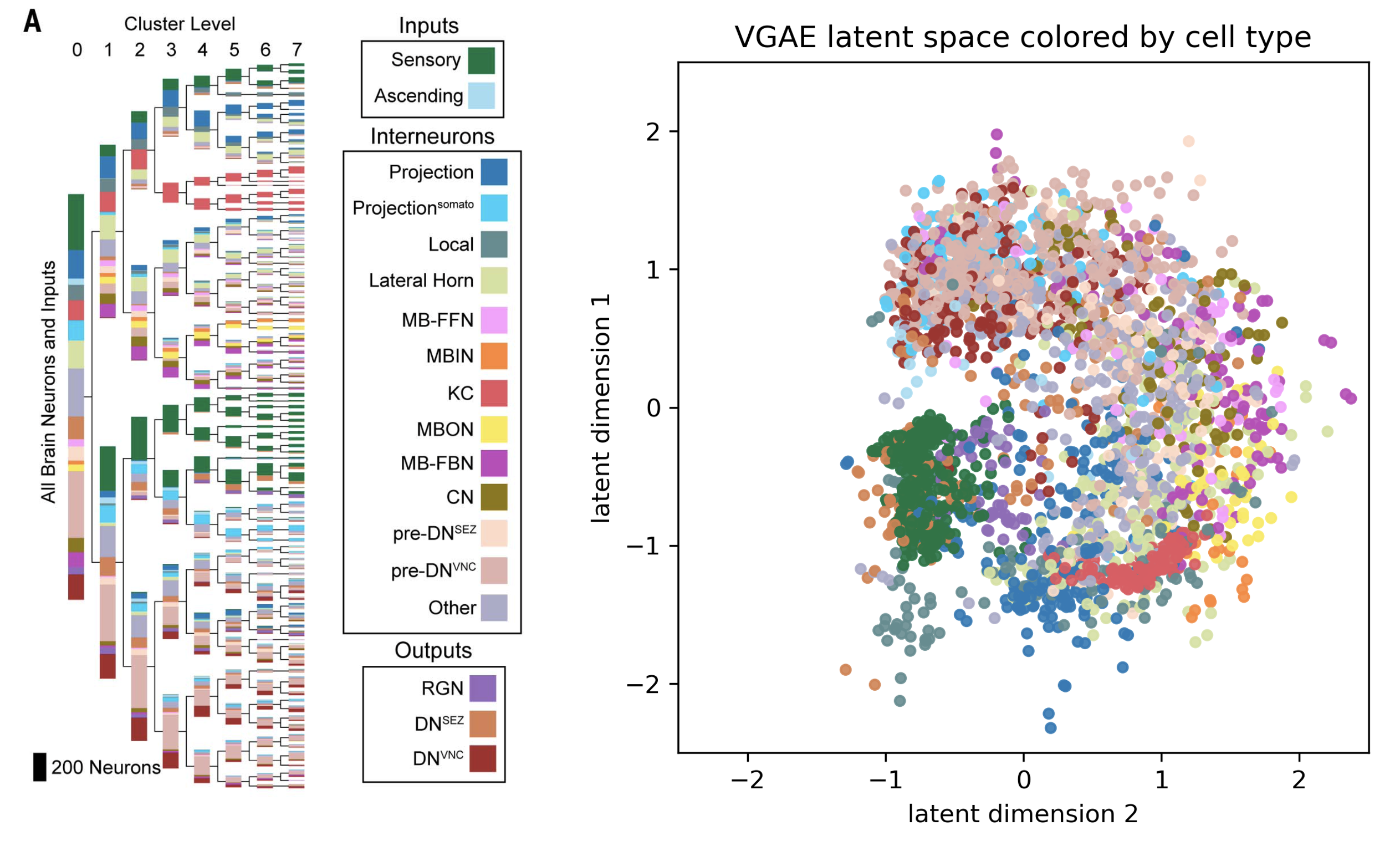
As seen in the figure above, both spectral embedding and GVAE latent spaces capture knowledge about the cell types when trained purely on the graph structure. We believe this is because cells of this type have similar properties in terms of the types of neighboring neurons they connect to in the connectome, and they may also have special properties like higher degree of connections.

In particular, it is interesting that sensory neurons and Kenyon cells are very well captured by both embeddings, and that MBIN cells and sensory neurons are clustered together by both their spectral embedding algorithm and VGAE.

Discussion

Our preliminary investigations show that deep learning algorithms such as Graph Autoencoders (GAEs) and Variational Graph Autoencoders (VGAEs) are able to capture at least as much nuance and information about function as spectral embedding algorithms. In addition, they come with the following advangates:

1. With their current implementation, they can easily be run on a GPU, while common spectral embedding algorithms in libraries such as scikit learn are only designed to work on CPUs. Since we take a deep learning approach, our GNN method can use batches optimized via Adam, while spectral embedding only works if the entire adjacency matrix fits in memoruy. This makes deep learning methods better able to scale to larger datasets such as the mouse connectome that may come in the next few years.
2. As shown in experiment 2, GAEs and Variational GAEs are able to directly learn a robust embedding into a 2-d space without any additional clustering, making interpretation easy and fast. We suspect that because of its higher performance at embedding connectomes to such low dimensions compared to spectral embedding which performs only marginally better than a random algorithm at such low dimensions, VGAEs must be capturing some addiitonal nuance of the graph structures that spectral embedding is simply not able to encode.
3. Comparing the 2-d embeddings of VGAE to the clustered 24-d spectral embeddings found in Winding et al. we find that even when compressing to such a low-dimensional space, the semantic information captured does in fact match that of spectral embedding at a higher dimensional space. Coloring by cell type shows that it also captures information about the function of neurons, with similar neuron types being clustered together even when they are located all over the brain, such as Kenyon cells. Cells of the same type likely serve simlar functions, so in this respect, VGAE is able to capture information about the function of cells using only knowledge of the graph structure.

However, VGAE does not come without its limitations. One large limitation we found while implementing the architecture is that it currently requires graphs to be undirected, so we had to remove information about the direction of neurons for this work. Connectomes are inherently directed, so we likely missed some key information about the function of graphs by removing this directional nature of the connectome. Although this is not explored in our work, one simple way to fix this would be to add features to each node corresponding to the in-degree and out-degree of each neuron.

This brings us to the another limitation of our study, which is that we did not explore adding features to neurons in our connectome with the VGAE algorithm. Past work on GAEs has shown that adding features leads to better model results and makes the model better able to capture relevant structures in the data. We did not feel that would be a fair comparison with Winding et al. because spectral embedding methods are not able to include additional features related to nodes that one would get for free when mapping the connectome, but we believe that including these features in the GAE structure would lead to an even better representation of the underlying dataset. Examples of these “free” features we could get that would help us predict functions of neurons include 1) the hemisphere the cell belongs to (e.g., not in fruit flies, but neurons in the left brain of humans correspond to language), 2) the axon I/O ratio, and the dendrite output-input ratio of a neuron.

One final limiation is that our model only trains on a single connectome. This means that we aren’t able to capture the variation of connectomes within a species. Maybe one day, we will be able to scan connectomes of people in the same way that we are able to scan genomes of people, but that day is likely still far away. We might be able to help this by using the generative compoment of the VGAE to create brains that are physically feasible given the structure of a single connectome, but it would be hard to test. Since we are currently only looking at the connectome of a single species, we likely aren’t capturing an embedding space that finds functionally similar neurons in different animals such as C. elegans, which we may be able to do in future work.

Conclusion

In this work, we asked if Deep Learning techniques like Variational Graph Autoencoders could learn something about the functions of cells in a connectome using only the graph structure. We found that VGAE did in fact capture relevant structures of the graph, even in the undirected case. It performed similarly to spectral embeding, even when embedding directly into a visualizable 2-d latent space. In the future, we may be able to learn about neurons that serve the same purpose across species, or learn about the underlying low level syntactic structures like for-loops or data types that our brain uses to encode consciousness, vision, and more.