Learning a Lifted Linearization for Switched Dynamical Systems

A final project proposal for 6.s898 in fall 2023

Introduction

All models are wrong, but some are useful. —George Box

Deep neural networks are incredibly capable of generating models from data. Whether these are models that allow for the classification of images, the generation of text, or the prediction of a physical system’s dynamics, neural networks have proliferated as a favored way of extracting useful, predictive information from set of data . But while well-tuned and well-designed neural networks can demonstrate miraculous performance at a given task, raw accuracy is not the only measure of a model’s usefulness.

In robotics, the speed at which a model can be run and its explainability can be just as important as the accuracy of its predictions. Techniques such as model predictive control can enable remarkable performance even when they’re based on flawed predictive models . In practice, most of these models are linearizations of more accurate, nonlinear equations. Produced by considering low order truncations of the Taylor series, these linearizations can be run incredibly efficiently on modern computer hardware and are amenable to linear analysis techniques for explainability purposes.

Nevertheless, this kind of linearization has its own weaknesses. Chief among them is the inherently local nature of the approach: a Taylor series must be taken around a single point and becomes less valid further away from this location. As an alternative, lifting linearization approaches inspired by Koopman Operator theory have become more commonplace . These techniques seek to linearize a system by lifting it to a higher dimensional representation where the dynamics can be made to evolve linearly over time. While such models can suffer from the curse of dimensionality when compared to their lower-order Taylor series brethren, they can offer greater accuracy while still providing most of the benefits of a linear model.

\(f(x)|_{x=a}\approx f(a)+\frac{f'(a)}{1!}(x-a)\)

A truncated Taylor series makes use of the derivatives of a function around a point.

Deep neural networks have emerged as a useful way to produce these lifted linear models . An encoder is used to transform a system’s state into a higher dimensional latent space of “observables”. These observables are then fed through a linear layer which evolves the system forward in time: a linear dynamical model. In the literature, this approach has come to be known as Deep Koopman Networks (DKNs). We can see how these networks can learn lifted linear models for physical systems by considering a simple pendulum.

An example of a neural network architectured used to learn observables for a linear Koopman model, taken from

Performance of a DKN for predicting a damped, simple pendulum across a set of trajectories. On the left, the dotted lines represent the ground truth trajectories, while the lines connected by crosses are the predicted trajectories. On the right, the MSE of the trajectories for the full 30 time steps of data is presented.

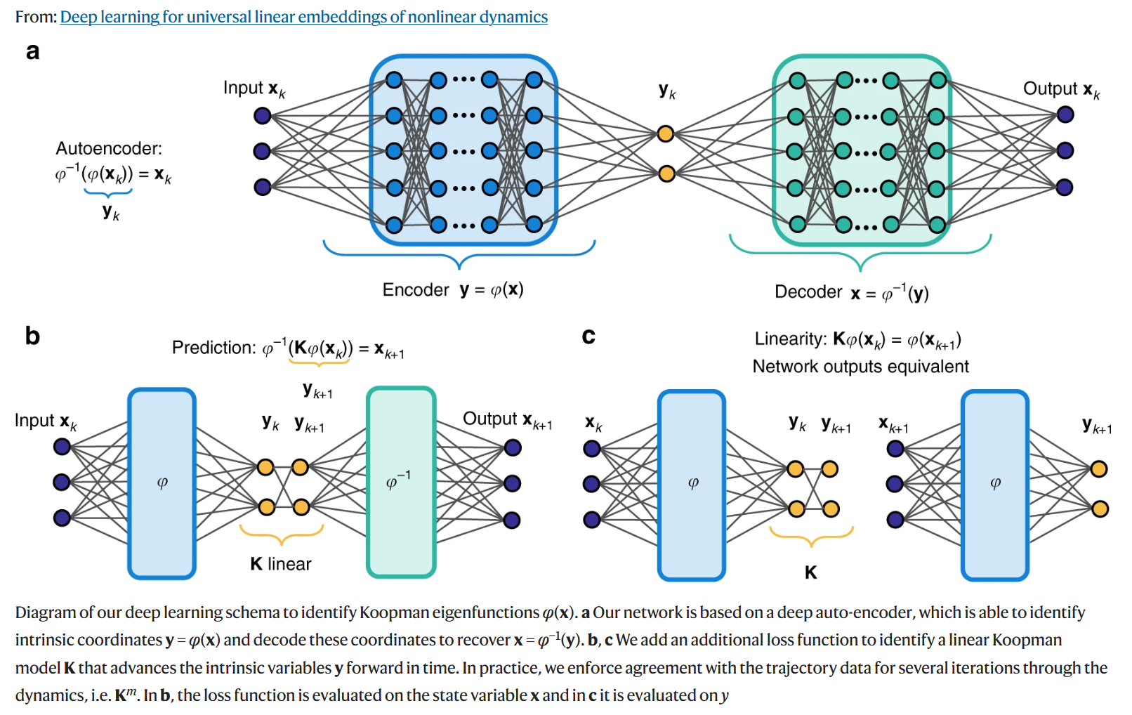
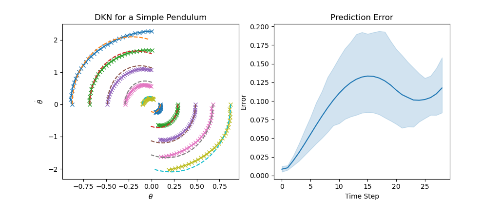
While the potential of DKNs has already been explored in recent years, the field is still being actively studied. In this blog, I am interested in exploring how a DKN can be used to model a particular kind of a dynamical system: one with piecewise dynamics that vary discretely across state space. These systems are inherently challenging for traditional, point-wise linearization techniques. To explain this, we can consider an example inspired by our old friend, the simple pendulum.

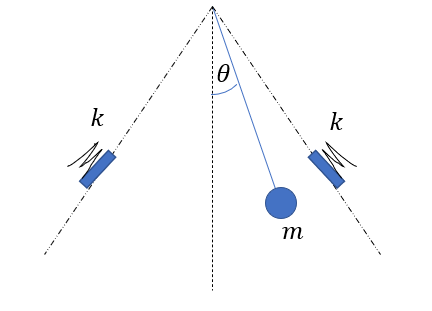
Consider a pendulum as before, but with the addition of two springs located at $\theta=30\degree$ and $\theta=-30\degree$. If we to consider a point arbitrarily close to one of these springs, say at $\theta=29.99…\degree$, then a Taylor series about this point – even with infinite terms – would not be able to accurately represent the dynamics when the spring is engaged. In contrast, a lifted linearization may better model such a system thanks to its ability to incorporate information beyond a single point.

\(\begin{align} \ddot\theta =f(\theta,\dot\theta) =\begin{cases} -g\sin{\theta}-b\dot\theta, & \theta\in [-30^\circ,30^\circ]\\ -g\sin{\theta}-b\dot\theta-k(\theta+30), & \theta<-30^\circ\\ -g\sin{\theta}-b\dot\theta-k(\theta-30), & \theta>30^\circ \end{cases} \end{align}\)

The dynamics of a pendulum with a pair of springs can be expressed as a set of piecewise equations. $k=1000$ is the stiffness of the springs and $b=1$ is the damping constant.

Diagram of the damped pendulum system with a pair of fixed springs, space at equal angles away from $\theta=0$.

Although that isn’t to say that a brute-force implementation of a DKN would necessarily be all too successful in this case either. Piecewise, switched, or hybrid systems (terminology depending on who you ask) are composed of particularly harsh nonlinearities due to their non-continuous derivatives. These can be difficult for lifted linearization approaches to model , with some systems theoretically requiring an infinite number of observables to be accurately linearized. This project is motivated by the question of whether we could modify the standard DKN approach to be more amenable for piecewise systems, specifically by taking inspiration from the common practice of pre-training neural networks.

As a bit of a spoiler for the conclusion of this report, we don’t end up seeing any noticeable improvement from pre-training the DKN. Nevertheless, the process of experimenting with the proposed approaches was an insightful experience and I am happy to share the results below.

Proposed Approaches

I experimented with two approaches for pre-training our DKN, one inspired by curriculum learning and another seeking to leverage an intuitive understanding of a lifted linearization’s observables. We then compared the results to an aggregate DKN model trained from scratch with 50 observables.

A DKN with 50 observables trained from scratch for the pendulum with springs. On the left, the dotted lines again represent ground truth trajectories while the lines connected by crosses are predictions.

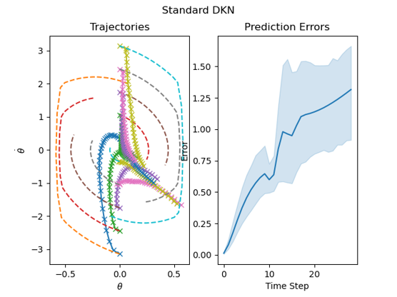
In the case of applying curriculum learning, we considered an approach with a data-based curriculum. In these cases, the difficulty of the training data is gradually increased over time. This has the potential benefit of allowing a model to more readily learn a challenging task, while also preventing a situation where a model is not sufficiently ‘challenged’ by new data during the training process. Our curriculum learning approach sought to take advantage of DKNs’ already good performance for the standard pendulum case. Intuitively, we identify the spring’s stiffness as the primary source of increased difficulty in our toy system. With this in mind, I created four data sets with different values for the spring constant, $k=0,10,100,1000$. A single model was then trained sequentially on these data sets. If our intuition is correct, we would expect to see the model gradually learn to account for the presence of the spring while maintaining the dynamics of a simple pendulum closer to the origin.

For the second approach tested in this project, it is necessary to consider what an observable is meant to represent in a lifted linearization. As an additional piece of terminology, the function which is used to generate a given observable is referred to as an observable function . While it may be possible to use different sets of observable functions to linearize a given system, it is possible to find a set of observable functions that are analogous to a linear system’s eigenvectors. The evolution of these observables in time, referred to as Koopman eigenfunctions, is defined by an associated complex eigenvalue. Much like their eigenvector cousins, these eigenfunctions can provide useful information on how the system might evolve over time, including information on how the time evolution may vary spatially.

Based on this understanding of Koopman eigenfunctions, we are motivated to see if a DKN could be coaxed into more readily learning spatially-relevant observables. If we consider our system of interest, the pendulum with springs, we posit that different regions of state space would be primarily influenced by different eigenfunctions. In particular, the larger central region where the pendulum’s dynamics are independent of the springs may be expected to be affected by a set of eigenfunctions with a lower spatial frequency and a global relevance. That is, eigenfunctions which better represent the dynamics of the system averaged throughout the state space and which may be valid everywhere – even when the springs are engaged, the natural dynamics of the pendulum are still in effect. In contrast, the dynamics when the springs are engaged (each spring is active in a comparatively smaller region of state space) may rely heavily on a set of eigenfunctions that are only locally relevant.

On the left, a visualization of trajectories used to train the models for the pendulum with springs. Dotted vertical lines mark where the boundary between regions of state space where the springs are and are not engaged. On the right, we see the trajectories considered for the system when there are no springs. Note that the presence of the springs compress `squeeze' the higher energy trajectories further away from the origin of the state space.

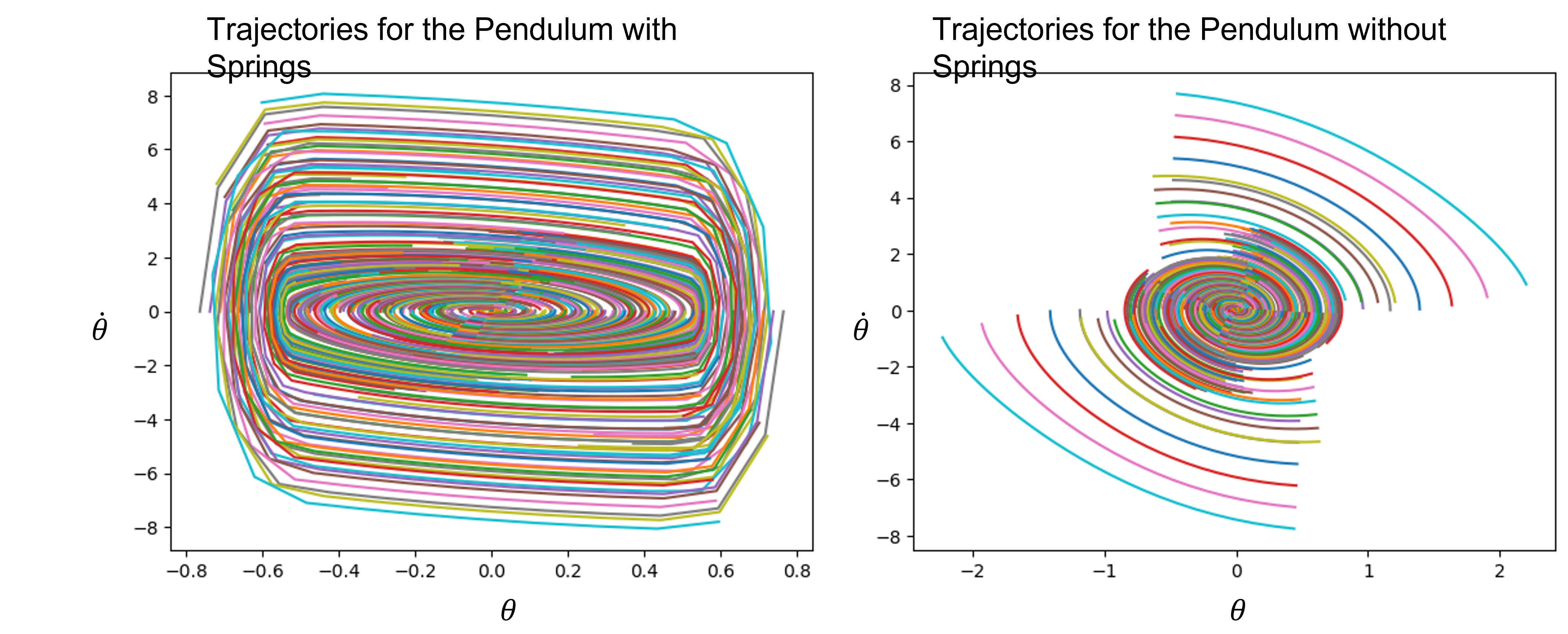
While I believe that this is an interesting thought, it is worth noting that this intuitive motivation is not necessarily backed up with a rigorous mathematical understanding. Nevertheless, we can empirically test whether the approach can lead to improved results.

In contrast to the curriculum learning approach, we have only a single set of data: that generated from a model of a pendulum with a spring stiffness of $k=1000$. Instead of the standard approach of DKN, where a larger number of observables is considered to (in general) allow for a system to be more easily linearized, we deliberately constrain the latent space dimension to be small. The intention is for this restriction to limit the number of observable functions that the model can represent, encouraging it to learn observables with a low spatial frequency and which are relevant across a larger region of state space. In our system of interest, this would be observable functions that represent the dynamics of the pendulum without the springs.

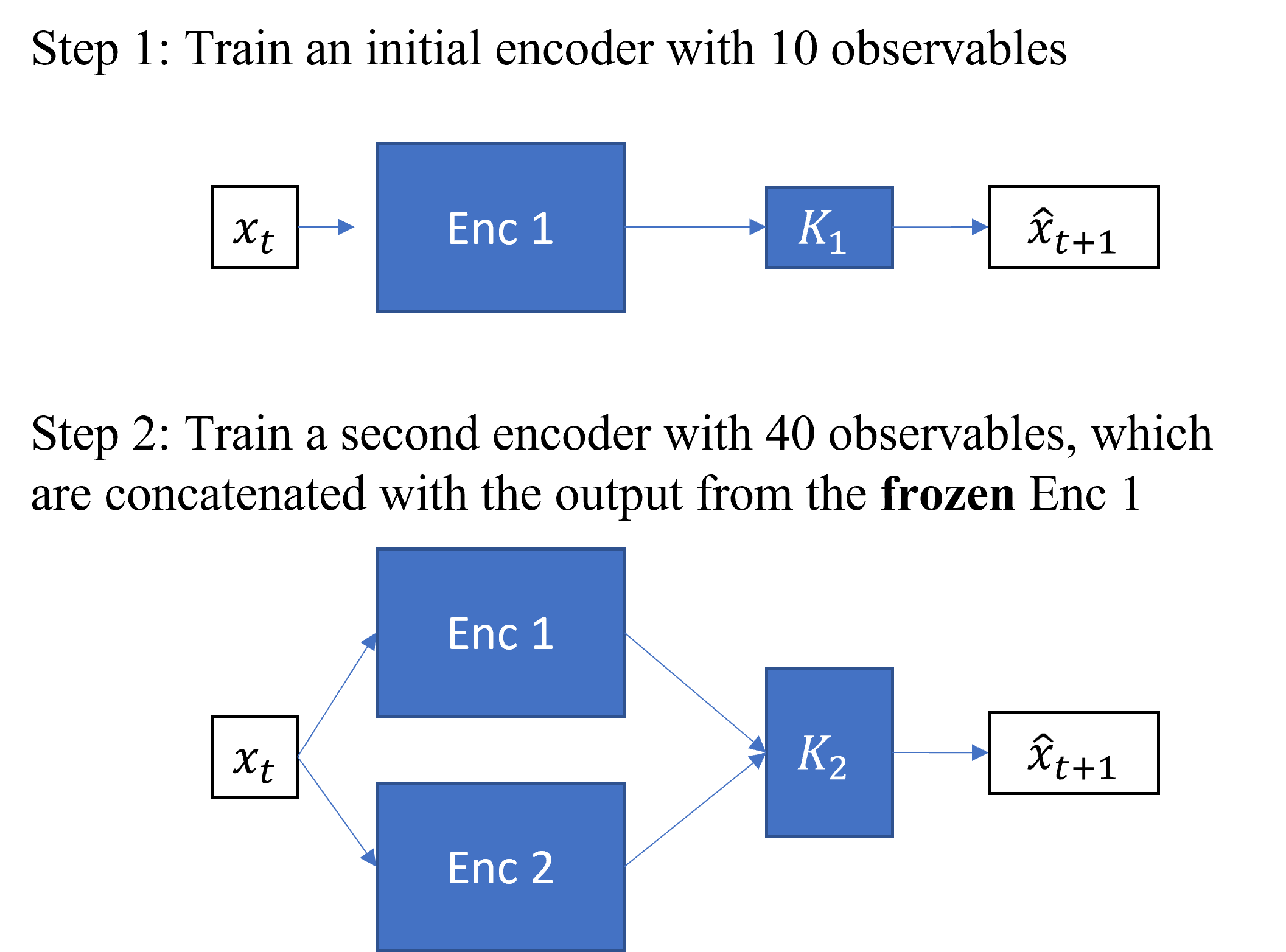
Once we have initially trained this smaller model, we use its encoder within a larger model. This initial encoder is kept fixed in future training processes so that it continues to represent the same set of observables. An additional encoder is then then in the larger model, with the goal being to learn additional observables capable of making up for the initial model’s deficiencies. If the initial model learned the low spatial frequency observables as hoped, then we would expect this additional encoder to learn observables that are more relevant in areas where the springs are exerting a force on the pendulum. In practice, we could see this as a particular form of curriculum learning where the complexity of the model is increased over time. A key difference here compared to traditional approaches is that instead of increasing the complexity of the model by adding layers depth-wise, we are effectively increasing the width of the model by giving it the ability to learn additional observables.

The architecture used to train the combined model. A smaller, 10 observable model was first trained, before a larger model was then trained to learn an additional 40 observables.

The Model

To reduce the influence that other factors may have in the results of our experiments, I sought to minimize any changes to the overall structure of the DKNs being used, save for those being studied. Chief among these was the number of hidden layers in the network, the loss function being used, and the input. Other variables, such as the optimizer being used, the batch size, and the learning rate, were also kept as unchanged as feasible. The need to tune each of these other hyperparameters and the challenges in doing so are well-documented in the machine learning field, and as such I won’t spend any additional time describing the processes involved.

The general encoder architecture of the networks being used was as follows, with $D_x$ being the number of states (2, in the case of the pendulum) and $D_e$ being the number of observables:

Layer	Input Dimensions	Output Dimensions	Nonlinearity
Linear	$D_x$	16	ReLU
Linear	16	16	ReLU
Linear	16	$D_e$	None

In addition to the encoder network, a linear layer was present to determine the time evolution of the observables. For this linear layer, the input and output dimensions were both D_e + D_x since our final set of observables always had the system’s states concatenated onto those learned by the encoder.

The loss function that I used was composed of two main components: a loss related to the time evolution of the observables being output by the encoder, and a loss related to the time evolution of the state variables. In the literature, additional loss terms are often included to help regularize the network during training. These were not found to be significant in the testing done for this report, however and so were excluded. Tests were also done with different weights between the state loss and the observable loss, with an equal balance between the two found to provide reasonable outcomes. Another hyperapameter that we needed to tune is for how many time steps to enforce a loss on the values predicted by the model. In this report, we stuck to 30 time steps although significant experimentation was not done to explore how varying this parameter may have affected the results. We did briefly look into whether having a weight on any of the loss terms which decayed over time would improve training and did not see any immediate benefits.

\(\mathrm{loss}=\mathrm{multistep\_loss\_state}+\mathrm{multistep\_loss\_observables}\) \(\mathrm{multistep\_loss\_state}=\sum^{30}_{t=1}\lvert\lvert(\psi(\textbf{x}_t)-K^t\psi(\textbf{x}_0))[:2]\rvert\rvert_{\mathrm{MSE}}\) \(\mathrm{multistep\_loss\_observables}=\sum^{30}_{t=1}\lvert\lvert(\psi(\textbf{x}_t)-K^t\psi(\textbf{x}_0))[2:]\rvert\rvert_{\mathrm{MSE}}\)

The loss function ultimately used for each of the models considers the prediction error for both the state and the observables. $\psi$ represents the act of using the model's encoder and then concatenating the state as an additional pair of observables. $K$ represents the linear layer in the architecture used to model the time evolution of the lifted state.

Analysis

Curriculum Learning

The initial model for stiffness $k=0$ was trained on the simple pendulum dynamics for 600 epochs, and served as the pre-trained model for this approach. Subsequent models were each trained for 200 epochs with the Adam optimizer and a decaying learning rate scheduler. When analyzing the performance of these models, we looked at how the error for a set of trajectories not in the training set evolved over time.

Performance of the model trained using curriculum learning after each of the learning stages. We observe that performance decreases over time, and that the original model trained when $k=0$ seems to perform the best.

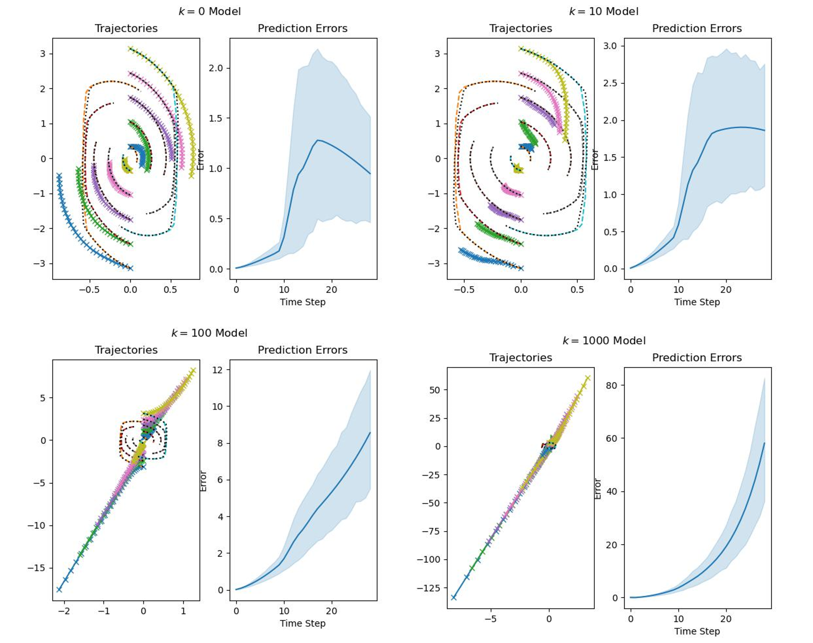
By this metric, we observe the performance of the model gradually getting worse. While this on its own is not too surprising, the final model ends up performing significantly worse than a DKN with the equivalent number of observables trained from scratch. Interestingly, it looks like the final model is unstable, with the trajectories blowing up away from the origin. Looking into this, issues surrounding the stability of linearized models is not a new phenomenon in the field of Koopman linearizations. Prior works have proposed several methods to help alleviate this issue, such as by adding an addition term to the loss function which stabilizes the time-evolution matrix. While there was no time to implement this change for this report, it could be an interesting modification to attempt for future work.

Learning New Observables

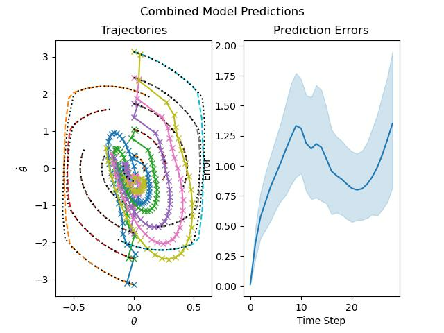
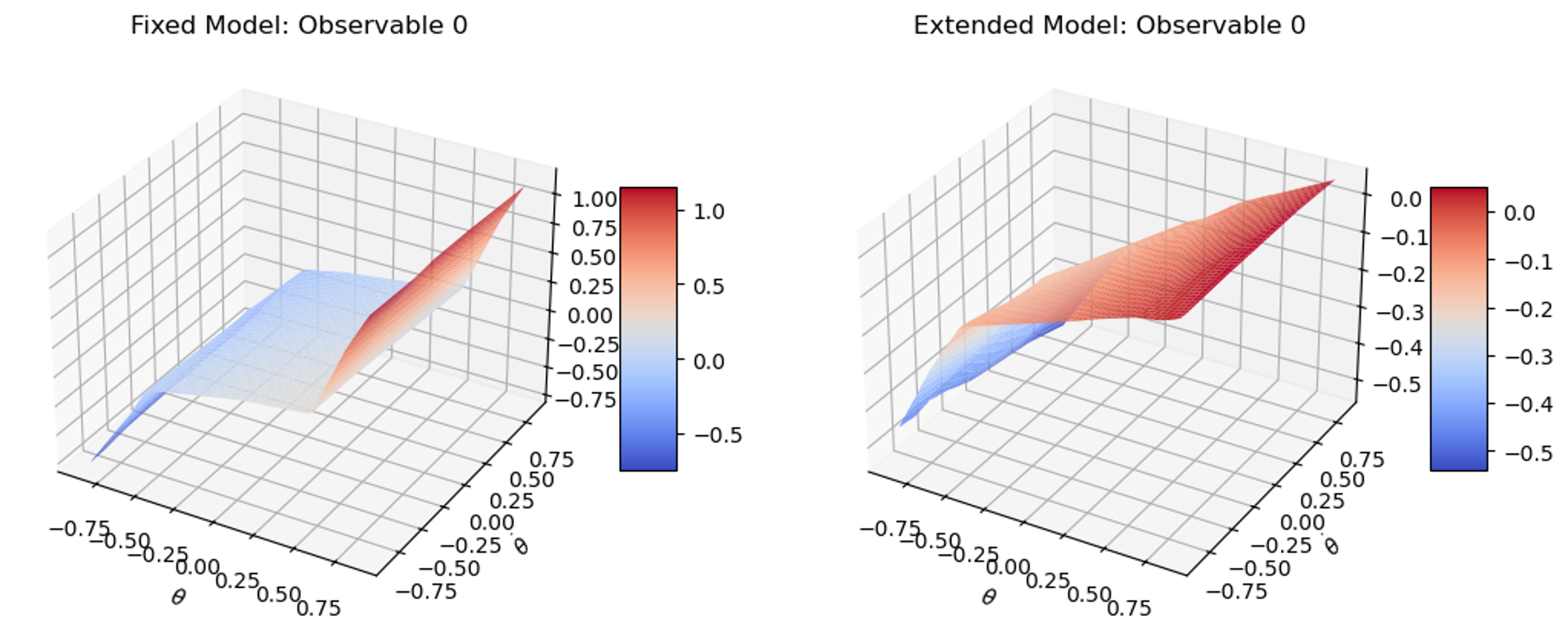
While trying to gradually learn additional observables for the model, we started with a network that learned 10 observable functions and trained it for 600 epochs. Once this process was complete, an extended model learned an additional 40 observable functions for an additional 600 epochs. The end result was comparable in performance to a single aggregate model of 50 observables trained from scratch. The aggregate model did appear to specifically outperform our gradually trained model during the initial time steps, while slightly underperforming in comparison at the later time steps. This may be due to some differences in the stability of the two learned linear models, although further investigation would be needed to verify this. Part of the motivation for this method was the hope that the network would learn locally relevant observable functions. The learned observables were plotted on a grid to visualize them and see if this were the case, but not distinctive, qualitative features indicating that different observables were learned for different regions of state space.

The combined model doesn't see any noteworthy improvement in performance when compared to the standard DKN approach. While not shown here, the combined model was found to be sensitive to how many observables were learned by each of its constituents. For example, having 30 observables in the first encoder and 20 in the second led to worse results.

Visualization of a pair of observables from the combined model, arbitrarily selected as the first observable from both encoder 1 (left) and encoder 2 (right). While only these two observables are shown here, plots for all 50 were produced. We noticed that observables from encoder 1 (the fixed model) tended to show `kinks' around $\theta=+-30\degree$. This may indicate that it was learning to account for the presence of the springs. In contrast, encoder 2 (the extended model) learned observable functions that were generally smoother across state space.

Conclusion

In this project, we sought to test two modifications to a DKN training scheme on an example of a piecewise dynamical system. By using a curriculum learning process or gradually increasing the number of observable functions, we hypothesized that the DKN would show better performance than an aggregate model trained from scratch. Ultimately, we found that neither of the proposed methods led to significant improvements.

One of the potential causes of underperformance is the learned linear models’ instability. While this is a known issue regarding lifted linearization techniques , attempting to resolve the issue would require further work and additional study into how best to do so for this use case. The example model of a pendulum with springs could also have been chosen poorly. I opted to experiment with this system since it was physically meaningful, and I believed that it would be a simple toy model that wouldn’t require large models with extensive compute requirements. But observing the dramatic change in performance that occurred in the linear models simply through the addition of the springs made me wonder whether this system truly was as simple as I had initially made it out to be. It is possible that larger and more elaborate models with more observables and resources for training are necessary to learn an appropriate linearization.

It is also worth considering the severe limitations of this study, imposed upon it by the need to tune a wide variety of hyperparameters. Even in the process of creating a linear model for the simple pendulum, I observed a wide range of performance based upon how the cost function or learning rate were varied. While some effort was taken to tune these and other hyperparameters for the models I explored, this process was far from exhaustive.

Moreover, the proposed changes to the typical DKN architecture only served to add additional hyperparameters into the mix. What spring stiffnesses should be used during curriculum learning? Should the learning rate be decreased between different curriculums, or should the number of epochs be varied? How about the ratio of observables between the two models used in the second approach, is a 10:40 split really optimal? Some variations of these hyperparameters were considered during this project, but again an exhaustive search for optimal values was impossible.

This means that there is a chance that I simply used the wrong selection of hyperparameters to see better performance from the tested approaches, it highlights the sensitivity that I observed in the performance of the DKNs. Even beyond the considerations described thus far, there are further considerations that can impact the structure and performance of learned linearizations. Some approaches augment the state variables with time-delayed measurements, for example. In other cases, the state variables are not included as observables and are instead extracted using a decoder network. This latter case is of particular interest, since recent work in the field has identified that certain types of nonlinear systems are impossible to linearize with a set of observables that include the states.

Ultimately, while the experiments in this project didn’t agree with my hypothesis (and resulted in some underwhelming predictive performance) I gained a newfound appreciation for the process of training these models along the way.