Exploring Image-Supervised Contrastive Diffusion - A Comparative Analysis with Applications in Image-to-Video Generation

Image-to-image (I2I) and image-to-video (I2V) may be the next frontier of generative deep learning capabilities, but current models struggle with robustness, largely due to the implicit, rather than explicit, representation learning objective during traditional diffusion model training. Hence, we propose a new technique where a custom contrastive loss function is used to leverage the innate latent space of the diffusion model’s variational autoencoder. This enables us to study the creation of lightweight models that lose less contextual information between input conditioning and target output, which we elucidate in this blog.

Introduction and Motivation

With recent advances in computer vision and generative AI, we all have observed the various feats that diffusive models have achieved in conditional image generation. These models have demonstrated unparalleled ability in creativity, fidelity, and relevance when generating images from text prompts. Given this explosive success of diffusion for the task of image generation, the idea of applying the same concepts to conditional video generation seems like a logical follow-up. Yet, the field still lacks robust and compelling methods for conditional video generation with diffusion models. This raises the question: why might this be? Or perhaps a follow-up: what makes videos so hard in comparison to images?

In an attempt to address our first question, if we take a brief dive into previous literature, we will find that the issue is not a lack of effort. Ho et al. , Zhang et al. , and Chen et al. , all explore this idea, yet the results from these methods are not nearly as exciting as the results we see in images. But why is this?

Perhaps the answer lies in the solution to our second question. One of the most obvious complexities that videos have over images is also perhaps one of the most difficult: the temporal dependence between frames. But why is this relationship so hard for diffusion models? Following the work of Zhu et al. , we hypothesize that this is because the implicit learning of diffusive steps between images in a video is too complex of a problem for a diffusion model; relying on the model to learn the implicit relationship between representations of video frames is infeasible from a training and convergence standpoint. If we can instead learn diffusive steps over a more regularized learned latent space, the optimization problem can be greatly simplified and the diffusion model will in theory be more robust.

To do so, we introduce a new framework for fine-tuning diffusion models when given images in addition to text as conditional information, targeting this challenge of making the model’s use of the latent space more robust. Specifically, we utilize contrastive learning techniques to ensure that the model learns consistency between latents from different image domains, which we first validate on the easier image-to-image (I2I) case before moving into image-to-video (I2V).

Related Work

Taking a step back to examine the current state of research, let’s first take a look at what current I2I models look like.

Image-to-Image Models

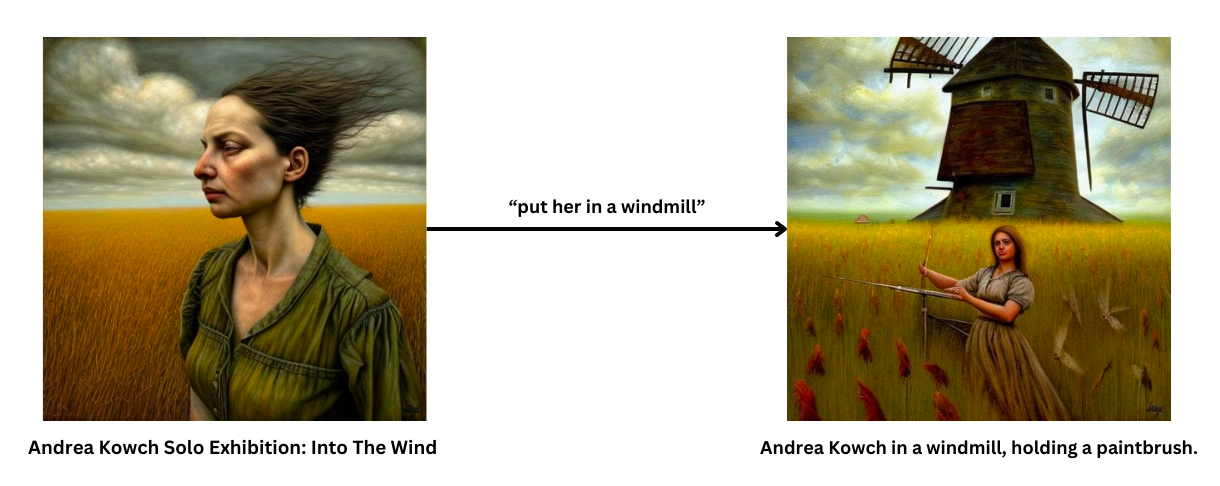
In the field of image-to-image, there are two main approaches, using images to control the model output, and modifying the image itself.

The first approach is characterized by work like ControlNet and T2I , which freeze the overall diffusion network and instead fine-tune a lightweight adapter model on the top. This adapter is typically a combination of stable diffusion layers that have an additive effect on the model as a whole, trained using the fine-tuning dataset. However, these models are largely still built for text-to-image tasks, using the input images as conditioning for the input text prompt, such as a wireframe image for poses. However, this does not allow modification of the image itself, simply using the image as guidelines during the diffusion process itself, meaning that its’ style is not preserved.

The second method is more related to maintaining both the style and content of the original image, and instead directly fine-tunes the diffusion network to actually use the input images. The first such model for this purpose is the original pix2pix architecture, which while built for GANs, still carries vital lessons to this day. By fine-tuning a loss that actually involves the mapping between input and output image, the model learns to actually adapt the image while keeping other relevant contexts the same . After this, the Palette model for generalist, multi-task diffusion trained a diffusion model from scratch for multiple different tasks . However, then Instruct-Pix2Pix built on the original pix2pix architecture, taking a pre-trained diffusion model and conditioning it on both the noisy text latent and the input image latent, meaning that the training latent had both and therefore would fully train on the input image latent . This architecture is presented below.

Traditional diffusion architecture

For the purpose of this blog, we study Instruct-Pix2Pix like fine-tuning schemes, since they align with what we need for video-based studies, maintaining content of the previous image while making small modulations based on the input text.

Image-to-Video Models

Moving to I2V, we find that current image-to-video frameworks typically still use a traditional diffusion architecture, going straight from text and image representations to an output image. However, this naive approach struggles with serious issues like frame clipping and loss of contextual information, which is expected since noise-based sampling can easily throw off the output of individual frames.

Hence, Ho et al. in 2022 proposed the first solution, supplementing conditional sampling for generation with an adjusted denoising model that directly forces image latents to be more similar to the corresponding text latents . While this achieved improved results over the straightforward diffusion approach, this often forces the model to stick too closely to the text latent, resulting in incoherent videos.

To solve this issue, two recent approaches from Chen et al. and Zhang et al. have proposed methods to augment the video diffusion models themselves. Chen et al. uses the image encodings from CLIP-like language embeddings in an encoder-decoder language model, feeding the CLIP encodings at each step into a cross-attention layer that generates attention scores with the current video generation . In doing so, additional coherence between frames is achieved. On the other hand, Zhang et al. use multiple encoders, with CLIP and VQ-GAN concatenated before two stages of diffusion model training, which they claim provides the hierarchical learning required to learn the temporal processing . However, both these models are extremely data-heavy and still suffer from hallucination and frame skipping.

Contrastive Models

To remedy these issues in diffusion models, Ouyang et al. and Zhu et al. posit that the implicit representation learning objective in diffusion models is the primary cause of the slow convergence and hallucination issues. Specifically, diffusion models do not directly compare their output to their input, as in contrastive models, instead performing a variational approximation of the negative log-likelihood loss over the full Markov chain. Instead, Ouyang and Zhu propose to train the diffusion model to output a structured latent in the latent space of a contrastive model like a VQ-VAE, which then reconstructs the output image . In doing so, a contrastive term can be added to the loss of the diffusion model, maximizing the mutual information between the structured (output) latent and input latent, leading to stronger correlations between input and output, and hence improved convergence. Hence, this approach seems to have potential in fixing the hallucination and coherence issues in video diffusion models, without the need for added complexity.

Our Proposal

Thus, we propose a novel method for conditional image-to-image generation (generating images given a starting frame and text description) by training the diffusion model to actually utilize the regularized latent space in which a diffusion model can operate. Following the line of thought introduced above, we hypothesize that under such a formulation, the diffusion model is much more robust to temporal inconsistency, because of the regularity in the latent space. For example, if we imagine a highly regularized latent space, we will find all logical next frames for a given anchor frame clustered very closely around the anchor in this latent space. Therefore, any step the diffusion model takes would produce valid subsequent frames; it suffices simply for the model to learn which direction to go given the conditioned text prompt.

Model Architecture

Image to Image

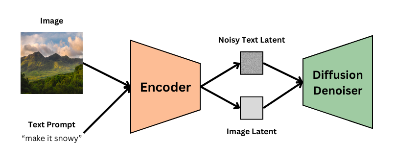
Given a base pretrained diffusion model, such as Runway ML’s StableDiffusion 1.4, which is the model used in this blog, it consists of various components. The three that are the most important are the VAE image encoder/decoder, the UNet, and the CLIP text encoder. The VAE begins by learning to transform images into latents and vice-versa, which is used to compress the input image and decode the output latent in the original Instruct-Pix2Pix stack. On the other hand, the UNet predicts the noise in the denoising part of the pipeline, whereas the CLIP text encoder encodes the input text.

In terms of the general diffusion model, we use the traditional diffusion loss,

\[\mathcal{L} = \mathbb{E}[(\epsilon - \epsilon_\theta(x_t))^2]\]

which essentially encodes the mean squared error loss between the added noise and the noise that is predicted by the UNet. This pipeline is illustrated in the below image.

Construction of the MSE loss for a traditional diffusion fine-tuning stack.

However, this loss does not encode anything of the relation between the frames themselves, which has the potential to lead to low coherence between source and target image, and thus lead to poor output quality. However, contrastively trained models like CLIP have shown strong correlative behavior between multiple modalities in the past, like between text and image, which is why we move towards contrastive losses.

In traditional contrastive learning, we typically have our classes divided by our dataset, such as for shape, as shown in this example of a shape dataset taken from the fourth homework of 6.s898:

An example of a contrastive dataset for shapes

For this contrastive learning dataset, we have images that are well classified, but in terms of our image to image task, there is no such easy classification. Instead, we adopt the notion that in such a dataset, with a batch size that is small relative to the size of the dataset, each image will be reasonably different from the other images. Also because we don’t want to cluster the latent space, as the VAE is fully pretrained in the case of the diffusion fine-tuning methodology, we don’t need to actually push similar items between the test set closer together, only push the diffusion output closer to the input conditioning.

Hence, for this task, we consider each image within the larger batch as a negative sample, only using the corresponding latent in our optimization task as the positive sample. Also, given that we want both similarity to the input image and the target image, we want our loss to look like

\[\mathcal{L} = \mathcal{L}_{MSE} + \mathcal{L}_{c, i} + \mathcal{L}_{c, t}\]

where c indicates contrastive and i, t indicate input and target, respectively.

For the images, they are encoded by the VAE, which has learned structure due to its Gaussian training objective in the ELBO loss, which means we can directly dot product the latents when calculating the contrastive loss:

\[\mathcal{L}_c = \mathbb{E}[\frac{e^{x_+^{T}x}}{\sum_{x' \in \{x_+, x_{-} \}} e^{x'^{T}x}}]\]

This is calculated easily using a matrix multiplication and a cross entropy loss. Now, since we compute the contrastive loss using the predicted latent, and not the noise, we also add on a constructive aspect to our diffusion model. From the final noise prediction, the model also generates the predicted latent using the noise scheduler:

\[x_0 = \frac{1}{\sqrt{\bar{\alpha_t}}}(x_t \pm \sqrt{1 - \bar{\alpha_t}}\epsilon_\theta(t))\]

where alpha is the cumulative products of the alphas in the noise scheduler. These predicted final latents are then used directly in the contrastive loss formula. A visualization of how we calculate our contrastive loss can be found below:

Construction of the MSE + Contrastive loss for our fine-tuning stack.

We note that in this case, we must scale the losses for numerical stability. The model we train with has latents of dimension 4 by 32 by 32, and while the MSE is scaled from 0 to 4 (due to pixel values from 1 to -1), the cross entropy loss is not. Indeed, many of these dot products are on the order of 4000, so we choose a high temperature of 1 to prevent NaN computations and then scale the losses by 4000, which is chosen because it scales the effect of each pixel in the dot product to around the same order as that in the MSE, which is averaged over all 4096 values in the latent.

Image to Video

Now, for image to video, the training process of such a model involves the optimization of the above diffusion/contrastive loss based on a given pair of nearby video frames, as well as the corresponding text description for that video. This procedure works well because in a video, we must train the model to learn the next frame, so just like how masked language models are asked to predict masked tokens from a sequence, we ask the diffusion model to predict a masked frame from the given frame. On top of that, the text prompt, which often still provides the majority of the guidance for the video as a whole is already conditioned using the MSE loss, while the contrastive loss optimizes the similarity to previous frames. Otherwise, this is trained the same as a traditional diffusion model.

During inference, we generate a video through the following process. First, an initial frame and the text description are encoded into our latent space using the VAE encoder and CLIP encoder, respectively. Now, we run an arbitrary number of passes through our diffusion model, generating a latent at each step, which is then passed in as the conditioning frame for the next forward pass. Finally, we decode the latent at each time step to obtain our video frame at that time step; stringing these frames together produces our video.

From a more theoretical perspective, this method essentially aims to restrict the diffusion model’s flexibility to paths within a highly regularized, lower dimensional latent space, as opposed to the entire space of images that classical diffusion-based approaches can diffuse over. Such a restriction makes it much harder for the diffusion model to produce non-sensible output; the development of such a method would therefore enable the robust generation of highly temporally consistent and thus smooth videos. We also imagine the value of producing such a latent space itself. An interesting exercise, for example, is taking an arbitrary continuous path along vectors within a perfectly regular latent space to obtain sensible videos at arbitrary framerates.

Data

Now, we explain where we got our data from.

For text-conditioned image-to-image generation, we train on the Instruct-Pix2Pix dataset from HuggingFace, sampling 20k samples from the original training set used in the paper (timbrooks/instructpix2pix-clip-filtered). Our test and evaluation sets consist of 500 nonoverlapping samples from this same set . This dataset consists of samples with input images, edited images, input prompts, edited prompts, and an edit string that describes the edit that was made. An example is presented below:

An example of a sample from the Instruct-Pix2Pix dataset.

For text-conditioned image-to-video generation, we experimented with the use of two different video-caption datasets: MSR-VTT and WebVid-10M. Due to the high dissimilarity between the properties of the two datasets, we tested the finetuning performance of both our contrastive model and non-contrastive models on both datasets. MSR-VTT contains 10k clips scraped from a wide range of domains, with multiple human-generated captions for each video. WebVid, on the other hand, contains 10M video clips compiled from stock image sources, with captions corresponding to the stock photo titles. For WebVid10M, we only take from the 2.5M subset. For both datasets, samples were generated to follow the Instruct-Pix2Pix data formulation (original image, edit prompt, edited image) using the following strategy:

First, we sample 25k and 10k videos from WebVid-10M and MSR-VTT, respectively. We aim to sample roughly an equal number of samples from each video for a total of 20k (original image, edit prompt, edited image) triplets. We ignore videos longer than 30 seconds in length to minimize the probability of temporal inconsistency within a given video. Then, for each video, we choose a random frame in the video (the original video fps is 25; but these frames are too close together, so we say that only one out of every 5 video frames is a valid selection target) to be our “original” image. The video’s caption is our “edit” prompt. To select our “edited” image, we note that we are optimizing the model to produce the next frame, while maintaining consistency between frames. Therefore, to select the “edited” image, we sample a normal distribution with standard deviation of 10 valid frames (50 frames in the original video), or two seconds, to select a frame after our “original” image as our “edited” image. A sample processed image from WebVid is included below.

An example of a processed sample from WebVid.

Experiments

To assess the efficacy of our newly proposed strategy, we run experiments on both the original Instruct-Pix2Pix task of text-conditioned image-to-image generation, as well as the task of text-conditioned image-to-video generation, against the baseline Instruct-Pix2Pix model. The original Instruct-Pix2Pix task is run to confirm that our model, after obtaining coherency, does not lose significant expressivity. On the other hand, we expect the image-to-video model to have comparable expressivity to the baseline on a task where coherency is significantly more important.

All of these evaluations and experiments were performed using the Accelerate library and HuggingFace Diffusers, , building off of their Instruct-Pix2Pix codebase. The model is RunwayML’s Stable Diffusion v1.5 release. For the task of image-to-image generation, we trained both the baseline Instruct-Pix2Pix and our model for 9000 training steps on 4xA100-80GB with a batch size of 16 and a learning rate of 5e-5, which took on the order of 12 hours. For the image-to-video generation task, we trained both baseline Instruct-Pix2Pix and our contrastive model for 4500 training steps at a learning rate of 1e-5 and a batch size of 16 due to overfitting issues at higher # of training steps and higher learning rates, possibly due to the repetitiveness of our dataset. Note that we had a limited ability to hyperparameter tune/ablate, since each diffusion fine tuning run took multiple hours at a minimum, and we were operating on a minimal budget of spare A100s when they were available from our labs, so those results are not shown in this blog.

We then evaluate on the test splits of the corresponding datasets described above (for image-to-video generation, we evaluate on the test split of WebVid, since MSRVTT’s testing set has a number of non-corresponding video-prompt pairs and also very jittery videos).

Results

Now, we explain our results. For both tasks, we assess two metrics: the first is the Frechet Inception Distance (FID) between the target image and the predicted image. The FID calculates the similarity between the distribution of images and the distribution of generated images, so a lower FID is considered better, as the distributions are more similar. Note that since our models are still technically image-to-image models and not image-to-video at their core, to evaluate the base models we use FID instead of its video counterpart FVD. For our second metric, we use CLIP Scores between the source image and the edit prompt, the target image and the edit prompt, and the predicted image and the edit prompt for the source image, predicted image, source image description (from the Instruct-Pix2Pix dataset), and target image description. The CLIP score can be thought about as a measure of the similarity between the prompt and the image, with a higher score being better, referring to higher similarity.

These metrics are used to evaluate our base image-to-video models as well, as they both determine the amount of prompt following and fidelity we can determine in our videos.

Image to Image Results

For text-conditioned image-to-image generation, we observe that our models have these FID and CLIP scores:

	FID	CLIP (source - prompt)	CLIP (gen - prompt)	CLIP (target - prompt)
Ours	158.8	21.7	24.4	24.1
Baseline	142.4	21.7	24.4	24.1

Our model matches the baseline on CLIP score, meaning that our model exhibits similar prompt following characteristics as the baseline. On top of that, our FID is only slightly higher than the baseline, meaning that the expressivity has not decreased significantly. However, images do not have similarly robust coherence metrics, so we evaluate these qualitatively.

Coherence

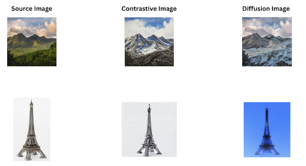
On the subject of coherence, we provide some image output pairs in the figure below:

An example of a sampled images, with prompt of "make the mountain snowy" and "make it futuristic," respectively.

For both scenes, while the baseline diffusion model follows the prompt more fully, which may match the output distribution (hence getting a better FID score), we notice several key contrastive differences, which would impact coherence. In the mountain for example, the forest disappears in the baseline version, which also doesn’t maintain the painting-like style. On top of that, in the Eiffel tower case, the Eiffel tower rotates in the non-contrastive version. These observations lead to the idea that the contrastive model may be prioritizing coherence as desired, despite some loss in performance. Similar patterns are observed throughout the dataset.

Image to Video Results

For text-conditioned image-to-video generation, we observe that our models have the FID and CLIP scores in the table below:

	FID	CLIP (source - prompt)	CLIP (gen - prompt)	CLIP (target - prompt)
Ours (trained on WebVid)	102.9	29.9	27.5	29.8
Ours (trained on MSR-VTT)	149.3	29.9	27.6	29.8
Baseline (trained on WebVid)	*	*	*	*
Baseline (trained on MSR-VTT)	172.3	29.9	**29.4 **	29.8

Note that in this case, we include asterisks for the baseline numbers on WebVid because it produces NSFW content as marked by the HuggingFace Diffusers library more than 25% of the time. This means that the metrics are not directly comparable as we were unable to find a validation set on which we could evaluate the models quantitatively on even ground. Nonetheless, we still include the WebVid baseline in our qualitative analysis.

Looking at the rest of the metrics, the baseline on MSR-VTT has a decently higher correlation with the prompt than the contrastive model. This makes sense, as the baseline is trained only the objective of denoising the prompt latent, while we add the contrastive term. On the other hand, we have a significantly lower FID score of the MSR-VTT trained models, which means that the distributions of our output data relative to the target output data was more similar, which is probably due to the fact that our high coherence is useful in tasks where source and target distributions are similar.

Qualitative Video Generation

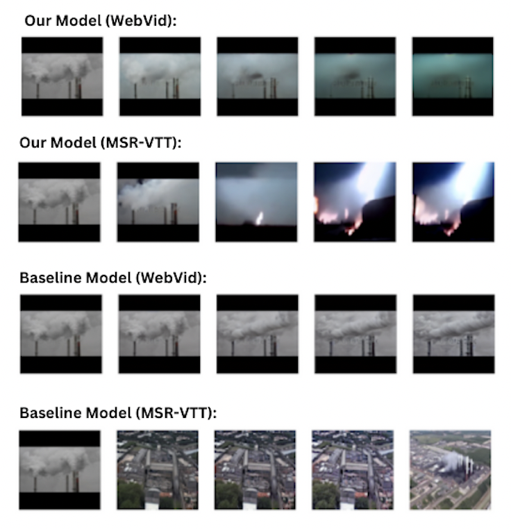
For a better understanding of the in-context performance of our model and to make up for the invalidity of the baseline model trained on the WebVid dataset above, we also perform qualitative assessments of longer videos generated by our models and the baselines. For each of 4 selected starting frames, we use a prompt generated from the sequestered part of WebVid to generate 5 subsequent frames for the video:

An example of sampled videos for a prompt of a factory emitting smoke.

From these generated videos, we observe that our models are significantly better at generating coherent frames, as we expected. In particular, we see that the MSR-VTT baseline model deviates heavily from the starting image on the very next frame, while our MSR-VTT model largely retains the original characteristics despite some content drifting after frame 3. WebVid noticeably performs better on the baseline, but does still observe some signs of progressive degradation in our predicted outputs, along with lack of motion in contrast to the prompt for the baseline model. This progressive degradation is likely due to small levels of inclarity in each subsequent frame being compounded over multiple frames; due to coherence between frames, the subsequent frames will contain strictly more inclarity than the previous. On the other hand, our model on WebVid sees less degradation on top of actually having coherent motion of smoke billowing, showing successful output.

Overall though, WebVid was observed to have significantly better results than MSR-VTT, which is likely attributed to the greater quality of the dataset and less jittery videos.

Discussion and Conclusion

In this project, we explored the idea of using contrastive losses to improve the coherency between input and output images in the context of text-conditioned image-to-image generation. In particular, we study the utility of this ability to generate highly coherent diffusion results in I2V, where the current state-of-the-art suffers heavily from temporal inconsistency. We evaluate our models on the classic Instruct Pix2Pix task to assess its preservation of expressive ability and conclude that no significant degradation of expressive ability was observed. We then evaluate our contrastive strategy on text-conditioned image-to-video synthesis and find that our models outperform the classic non-contrastive formulation in video generation tasks when evaluated on CLIP Score and KID.

Through our experiments, we have also identified some limitations of our methods and potential areas for improvement. First, we note that our model has trouble with the previously mentioned problem of progressive degradation. A possible solution to this problem could be introducing GAN training to encourage the model to produce higher-fidelity images. More robust methods could also be used (instead of sampling subsequent frames) to generate positive samples, which would increase our model’s robustness. We also notice that both our model and the baseline have trouble with a continuous depiction of motion. This is likely due to the fact that any frame is only conditioned on the previous frame. Conditioning on images multiple frames before the current image would help with this consistency issue, as well as the aforementioned progressive degradation issue. Also, due our loss function’s negative sampling-based approach to training our models, on a dataset with significant amount of repetition like ours, this led to significant overfitting in preliminary runs. On top of that, runs suffered from loss spiking when the numeric instability of cross-entropy loss led to the calculation of NaN losses and exploding gradients, which leads to requiring very low values of learning rate. This could be resolved with better sweeps of hyperparameters for scaling the losses relative to each other or higher quality data. Finally, as alluded to above, more time to do hyperparameter tuning with the training of larger models on larger datasets would likely help with performance in general.

With this study, we examined the use of contrastive loss to improve coherency in latent diffusion, with experiments that demonstrated minimal loss of expressive capabilities and superior consistency in diffusion, resulting in better performance on image-to-video generation. We hope that through this study, we can drive focus toward contrastive loss approaches to obtain higher fidelity results in video generation, accelerating progress in I2V and T2V.