To Encode or Not To Encode: The Case for the Encoder-free Autodecoder Architecture

While the traditional autoencoder architecture consists of an encoder and a decoder to compress and reconstruct information with only the most prominent features, some recent work have begun to utilize an alternate framework, the autodecoder, in specific applications in the field of representation learning. Skipping the encoder network altogether and learning latent codes directly as parameters, we aim to compare the two architectures on practical reconstruction tasks as well as dive into the theory of autodecoders and why they work, along with certain novel features that they bring.

Autodecoders

Introduction

Autoencoders have been a part of the neural network landscape for decades, first proposed by LeCun in 1987. Today, many variants of the autoencoder architecture exist as successful applications in different fields, including computer vision and natural language processing, and the variational autoencoder remains among the forefront of generative modeling. Autoencoders are neural networks trained to reconstruct their input as their output via compression through dimensionality reduction, accomplishing this task with the use of an encoder-decoder network.

Autoencoders comprise of the encoder network, which takes a data sample input and translates it to a lower-dimensional latent representation consisting of only the most necessary features, and the decoder network, which attempts to reconstruct the original data from this encoding. By learning a compressed, distributed representation of the data, the latent space learned by autoencoders is usable for a plethora of downstream tasks.

With traditional autoencoders, both the encoder and decoder are trained, but for certain applications— particularly generative tasks— only the decoder is utilized for inference. Because the itself encoder is not used at test time, training an encoder may not be an effective use of computational resources; the autodecoder is an alternative architecture that operates without an encoder network and brings some novel benefits.

Rather than using the encoder to encode an input into a low-dimensional latent code, each sample in the training set begins with a randomly initialized latent code, and the latent codes and decoder weights are updated jointly during training time. For inference on new data, the latent vector for a given sample is then also randomly initialized and updated through an additional optimization loop with the decoder’s frozen weights.

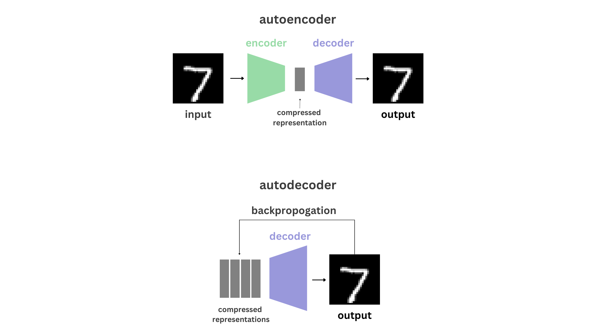
The architecture for an autoencoder (top) compared to that of an autodecoder (bottom).

Are explicit encoders necessary for image reconstruction? What are the unique benefits that come from using decoder-only architectures? One interesting application of autodecoders is the ability to reconstruct complete samples from partial inputs. The main focus of our research revolved around testing this ability, answering the question of how much of a sample is required for a complete reconstruction using an autodecoder given an expressive latent space, and comparing its performance to that of an autoencoder.

Furthermore, we discuss additional applications in various fields that other research has accomplished in part due to the utilization of the autodecoder architecture over the traditional autoencoder, with a focus on the beneficial properties that we explore in our experiments, including partial reconstructions.

Different literature have utilized autodecoder frameworks in the past along with providing rationale for their usage, mainly for tasks related to reconstruction or generative modeling through representation learning. However, none have provided standalone examples of their use, something we aim to accomplish in this blog.

The Generative Latent Optimization framework was introduced by Bojanowski et al. (2019) as an alternative to the adversarial training protocol of GANs. Instead of producing the latent representation with a parametric encoder, the representation is learned freely in a non-parametric manner. One noise vector is optimized by minimizing a simple reconstruction loss and is mapped to each image in the dataset.

Tang, Sennrich, and Nivre (2019) trained encoder-free neural machine translation (NMT) models in an endeavor to produce more interpretable models. In the encoder-free model, the source was the sum of the word embeddings and the sinusoid embeddings (Vaswani et al., 2017), and the decoder was a transformer or RNN. The models without an encoder produced significantly poorer results; however, the word embeddings produced by encoder-free models were competitive to those produced by the default NMT models.

DeepSDF, a learned continuous Signed Distance Function (SDF) representation of a class of shapes, was introduced by Park et al. (2019) as a novel representation for generative 3D modelling. Autodecoder networks were used for learning the shape embeddings, trained with self-reconstruction loss on decoder-only architectures. These autodecoders simultaneously optimized the latent vectors mapping to each data point and the decoder weights through backpropogation. While outperforming previous methods in both space representation and completion tasks, autodecoding was significantly more time consuming during inference because of the explicit need for optimization over the latent vector.

Sitzmann et al. (2022) introduced a novel neural scene representation called Light Field Networks (LFNs), reducing the time and memory complexity of storing 360-degree light fields and enabling real-time rendering. 3D scenes are individually represented by their individual latent vectors that are obtained by using an autodecoder framework, but it is noted that this may not be the framework that performs the best. The latent parameters and the hypernetwork parameters are both optimized in the training loop using gradient descent; the LFN is conditioned on a single latent variable. Potential applications are noted to include enabling out-of-distribution through combining LFNs with local conditioning.

Scene Representation Networks (SRNs) represent scenes as continuous functions without knowledge of depth or shape, allowing for generalization and applications including few-shot reconstruction. SRNs, introduced by Sitzmann, Zollhöfer and Wetzstein (2019), represent both the geometry and appearance of a scene, and are able to accomplish tasks such as novel view synthesis and shape interpolation from unsupervised training on sets of 2D images. An autodecoder framework is used to find the latent vectors that characterize the different shapes and appearance properties of scenes.

Methodology

Traditional Autoencoder

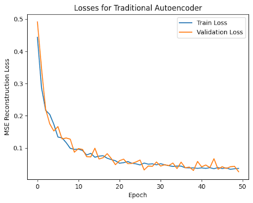
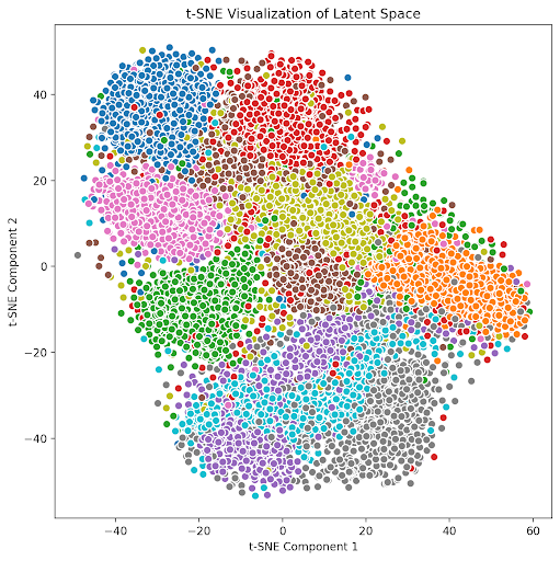
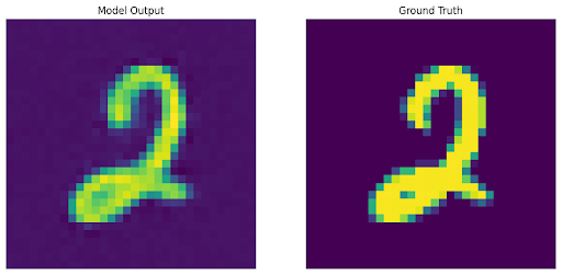
To establish a baseline, we first trained a convolutional autoencoder network containing both an encoder and decoder on a version of the MNIST dataset normalized and padded to contain 32x32 sized images. For our autoencoder architecture, we utilized convolutional layers with ReLU nonlinearity.

The training and validation losses from the training loop for the autoencoder.

The latent space learned by the autoencoder, color-coded by digit label and visualized through a 2-dimensional t-SNE plot. We see the expected result, with consistency and separation.

A sample output from an unseen image after training. We can see that our small convolutional autoencoder does a fairly good job at learning how to compress simple information into a single latent code and decode it into its original form.

Autodecoder

We implemented and trained an autodecoder on the same dataset by creating a convolutional decoder that takes latent codes as an input and transforms them into full images. We utilized transpose convolutions to upscale the images while additionally concatenating normalized coordinates to embed positional information, and also used leaky ReLU layers for nonlinearity.

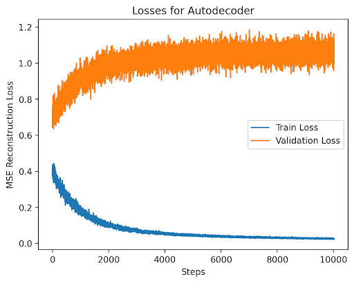
For training, the latent codes for 10,000 images in our training set were randomly initialized. The loss for our autodecoder then included three components: the reconstruction loss; the latent loss, which encourages latent values to be closer to zero in order to encourage a compact latent space; and the L2 weight regularization, which prevents the decoder from overfitting to the training set by encouraging the model weights to be sparse.

The loss function used to train the autodecoder. During inference, a custom loss function can be used based on the application.

The training and validation losses from the training loop for the autodecoder. The validation loss has no actual meaning in the autodecoder framework, as new images would have a randomly initialized latent code and so would output nonsense. This loss was included simply to demonstrate this feature.

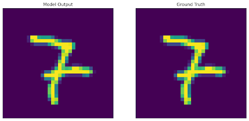
Below are progressive reconstructions on the training data performed by the autodecoder as it trained and optimized both the decoder weights and the training set’s latent codes. We can observe that the digits’ general forms were learned before the exact shapes, which implies good concentration and consistency of the latent space between digits of the same class.

Progressive reconstructions from top to bottom (model outputs compared to ground truth): 1. Decoding a randomly initialized latent code outputs nonsense. 2. The correct digit is reconstructed, implying that the latent space is improving, but the specific shape differs from that of the ground truth image. 3. The output’s shape begins to better match that of the ground truth. 4. The autodecoder and latent code are optimized to be able to effectively reconstruct the ground truth image.

The latent space learned by the autodecoder, also visualized through a 2-dimensional t-SNE plot. When compared to the t-SNE plot representing the latent space learned by the autoencoder, we again see consistency but notice that here the clusters are more compact. While the distance between clusters in t-SNE plots does not have a definite meaning, this could potentially imply that the features of shapes, rather than the shapes themselves, are better learned, as different digits share similar features (curves, straight lines, etc).

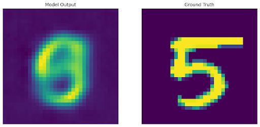
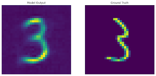
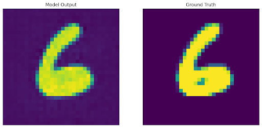
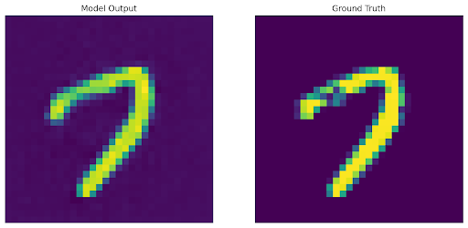
Upon training the autodecoder, for inference on a new image we first freeze the decoder weights and then run an additional gradient descent-based optimization loop over a new randomly initialized latent code with reconstruction loss.

Output from the trained autodecoder on a new image from the test set.

Experimentation

One benefit of the autodecoder framework is that because we have an additional optimization loop for each input during inference, we are able to do varying pixel-level reconstructions, whereas an autoencoder is designed and trained to reconstruct complete images each time.

We demonstrate this feature in our experiments below by applying center masks to our images before autoencoding or decoding.

1: We trained a traditional autoencoder with generic reconstruction loss, and input an image with a mask in the center. The output is expected, as the autoencoder learned to reconstruct whatever it saw, and so the empty space from the mask is included in the result.

The reconstructed image compared to the image without the mask.

2: We trained a traditional autoencoder with reconstruction loss without considering a centered square area and input an unmodified image. The output is again expected, as the autoencoder was trained to fully disregard the center area, and so the output is empty in that region.

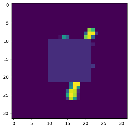
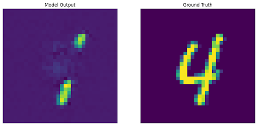
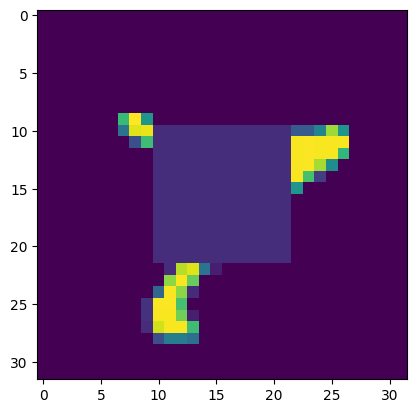
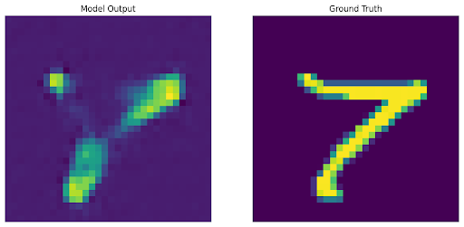
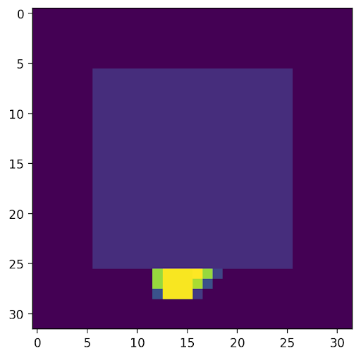
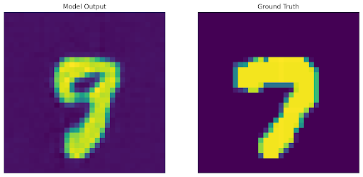
The area of the images that the autoencoder is trained to learn on.

The model output compared to the original image.

3: We trained an autodecoder with generic reconstruction loss, and during the optimization loop for inference we utilized a custom loss function that did not consider the masked area. However, in this case, we are still able to reconstruct the original image to varying levels of success because of the latent space we originally learned through the training loop.

Shown below are the areas optimized in the loss functions, along with the decoded output and original image.

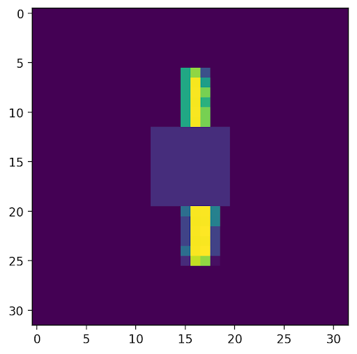
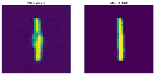
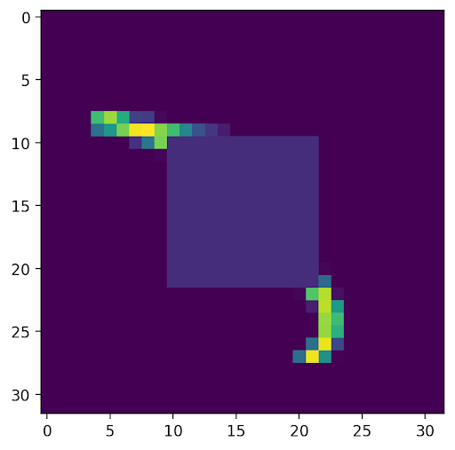
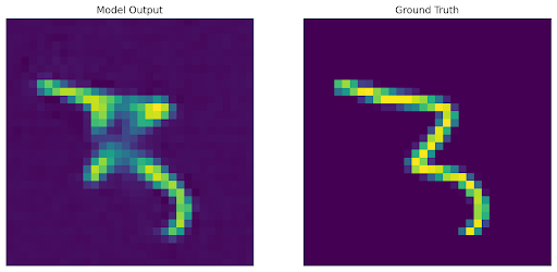
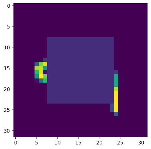
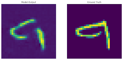
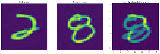
A 12x12 mask. Even with significant information about the digit missing, the autodecoder is able to sufficiently reconstruct the ground truth image based on the learned information.

A 20x20 mask. Although the reconstructed digit is ultimately incorrect, we see that we are able to get very close even with extremely limited inputs.

To analyze and compare the latent spaces learned by both our autoencoder and autodecoder, we additionally perform linear interpolation (with α=0.5) between the embeddings of two images and include their decoded results below.

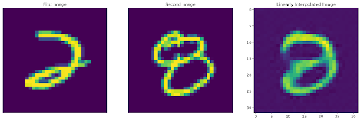
The output of the decoded interpolation of two embeddings from the autoencoder.

The output of the decoded interpolation of two embeddings from the autodecoder.

The autoencoder output was somewhat expected due to the simplistic nature of the MNSIT dataset, and we can see a merge of the two images with equal features of both.

More interesting was the output for the autodecoder, which simply returned an image consisting of the pixel average of both images. Some hypotheses for this result include:

The shape of the latent space for the learned autodecoder potentially being one that does not pair well with linear interpolation, causing linear interpolations in latent space to be equivalent to those in the data space. Meanwhile, the shape of the latent space for the autoencoder might better match a Gaussian, which translates to effective nonlinear interpolations in the data space, which is desired.
The inductive bias from the existence of the encoder architecture allowing for better interpolatability.

Conclusion

Discussion

While autoencoders (and variations such as VAEs) have traditionally been the standard architectures for representation learning, we explore an alternate autodecoder architecture, in which the encoder is excluded and individual latent codes are learned along with the decoder. We investigated the necessity of an explicit encoder in representation learning tasks and found that even without an encoder network, we are able to learn latent representations of input data through the optimization of randomly initialized latent codes during the training loop. Through this alternate dimensionality reduction process, we showed that we were still able to learn a consistent latent space on a multi-class dataset. Furthermore, we showed that through the use of an additional optimization loop for inference rather than learned encoder weights, the autodecoder can learn to reconstruct incomplete observations through pixel-level optimizations.

The autodecoder has the potential for many further applications beyond the scope of the research and experiments introduced in this blog. As an example, the task of prior-based 3D scene reconstruction in the field of computer vision, in which novel views of a 3D scene can be generated from a limited number of static images of that scene along with their camera poses, utilizes the autodecoder architecture to guarantee better out-of-distribution views. This task involves the use of camera pose as an additional source of information in addition to input images, something that the encoder itself is unable to integrate when encoding images, leading to the valuable scene representation information being left out. Meanwhile, because the latent code itself is learned in an autodecoder, it is able to use the camera pose to effectively generalize to novel viewpoints. This serves as just one of several examples of the autodecoder being able to carry out tasks normally gatekept by the limitations of the encoder.

Limitations

Some limitations of the encoder-free architecture include certain fallbacks discussed in our experiments, including the difficulties in generating satisfactory novel outputs through linear interpolation of the latent space. Furthermore, while the existence of a secondary optimization loop during inference comes with interesting properties such as being able to define unique loss functions for different purposes, this can be more computationally or temporally costly than running inputs on a trained encoder for inference. Regardless, as much of the research around this topic has emerged only within the past several years, it can be expected that autodecoders and their unique properties will continue to emerge, evolve, and find use in novel applications in the years to come.

References

Robin Baumann. Introduction to neural fields, 2022.

Piotr Bojanowski, Armand Joulin, David Lopez-Paz, and Arthur Szlam. Optimizing the latent space of generative networks. arXiv preprint arXiv:1707.05776, 2017.

Jeong Joon Park, Peter Florence, Julian Straub, Richard Newcombe, and Steven Lovegrove. Deepsdf: Learning continuous signed distance functions for shape representation. In Proceedings of the IEEE/CVF conference on computer vision and pattern recognition, pages 165–174, 2019.

Vincent Sitzmann, Semon Rezchikov, Bill Freeman, Josh Tenenbaum, and Fredo Durand. Light field networks: Neural scene representations with single-evaluation rendering. Advances in Neural Information Processing Systems, 34:19313–19325, 2021.

Vincent Sitzmann, Michael Zollhöfer, and Gordon Wetzstein. Scene representation networks: Continuous 3d-structure-aware neural scene representations. Advances in Neural Information Processing Systems, 32, 2019.

Gongbo Tang, Rico Sennrich, and Joakim Nivre. Encoders help you disambiguate word senses in neural machine translation. In Proceedings of the 2019 Conference on Empirical Methods in Natural Language Processing and the 9th International Joint Conference on Natural Language Processing (EMNLP-IJCNLP). Association for Computational Linguistics, 2019.