A Method for Alleviating Catastrophic Forgetting With Explainability
Using various explainability metrics to target, we freeze layers in CNNs to enable continual learning.
Introduction
With recent advancements in deep learning, the intelligence of computers is quickly rivaling that of humans. GPT-4, with significant size and data, is able to score in the 90th percentile of the BAR, 88th percentile of the LSAT, and the 92nd percentile on the SAT
The human brain is able to protect itself from conflicting information and reductions in performance on previous tasks using complex mechanisms involving synaptic plasticity
In contrast to the human’s ability to learn, neural networks significantly alter their parameters when learning a new task. In effect, the network’s understanding of previous tasks is overwritten. This poses a great barrier to the creation of artificial general intelligences, which ultimately depend on continual, life-long learning
With the rapid increase in size and complexity of models, the field of model explainability and the desire to understand exactly what models are doing has quickly grown. Specifically in the field of computer vision, effort has been made to understand how models make decisions, what information leads to this decision, and how they learn what to observe
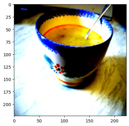
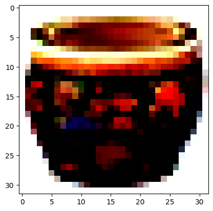
We propose to make use of these explainability methods for the intelligent freezing of filters of a convolutional neural network. Specifically, we use saliency maps and filter visualizations to consider what a model is observing to classify an image, and then decipher which filters are most strongly contributing to this. In this paper, we contribute the following: 1. We create a method for the ranking of importance of filters in a convolutional neural network. We expand and combine upon previous works in model explainability to understand which filters are most strongly contributing to positive predictions. 2. We create a method for the freezing of filters of a convolutional neural network according to these rankings. We do this by first training on one task, freezing filters according to importance, then retraining the same model on a novel task. In doing this, we both corroborate our ranking system and identify a new strategy for alleviating catastrophic forgetting.
Related Works
Continual learning and its core problem of catastrophic forgetting has gotten recent attention in deep learning research. It’s easy to understand why the goal of having a model that can adapt to new data without being completely re-trained is sought after, and there have been many approaches to the problem of aiding the model’s ‘memory’ of past tasks. Solutions range from attaching a significance attribute to certain weights in the model that regularizes change introduced by the new data to explicitly freezing weights via different metrics of the weights’ performance.
Weight Changing Regularization
Elastic Weight Consolidation(EWC) approaches the problem of catastrophic forgetting by adding a ‘stiffness’ to the weights of previous tasks dependent on an approximation of the importance they had to previous task performance. The authors of ‘Overcoming catastrophic forgetting in neural networks’
Another technique that attempts to use a regularizing factor to slow the retraining of old task parameters is explicitly computing a importance metric for each neuron in the network
Architectural Changes
A drastically different approach that a couple papers investigated was preventing interference between training runs by completely freezing the weights in parts of the model after completing a task’s training. The papers here differentiate themselves via the method they decide to freeze certain weights and layers. The earliest such paper we found was detailing a method called Packnet
Instead of simply measuring the magnitude of weights to decide what layers or specific weights to freeze, authors of a paper on catastrophic forgetting explainability paper use a custom metric to find a layer that scores highest on their metric and subsequently freeze all the layers prior to that layer
Explanability Metrics
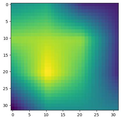
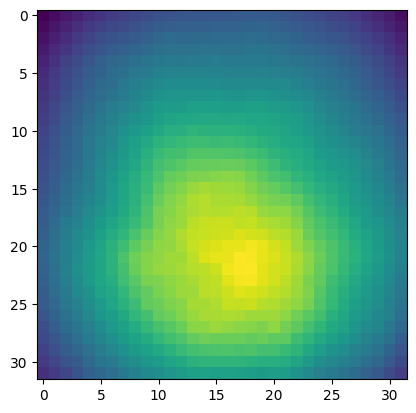
There exists many other explainability metrics with which one can target layers prior to training on a new task to try to prevent interference, an interesting one being saliency maps. Saliency maps attempt to capture the importance of features of the input on the output of a deep neural network. In the domain of CNNs, this can be thought of both the pixels and larger features, such as a window on a car, that contribute to a correct classification; saliency maps are analogous to trying to map out what parts of an image a model uses to make correct identification. A model of saliency maps we felt compelled enough to use in our project is that of
Methods
Model Type
We tested our method using VGG16. VGG16 is a deep convolutional neural network that has achieved impressive results on the ImageNet classification challenge, with a top-1 accuracy of 72%

Saliency Mapping
The computation of saliency maps is grounded in the principles of backpropagation. It follows a multi-staged procedure which uses gradients to consider the impact of each pixel in an image. First, it computes the partial derivatives of the target output with respect to individual segments of the input image. Then, it uses backpropagation to propagate error signals back to the input layer. It does this in order to identify the impact of pixels. It considers pixels with larger signals to have the greatest impact on the decision-making process. There are a bountiful number of papers which propose different improvements on the original saliency map. When selecting a procedure, we identified two key features necessary for a useful visualization. We believed that a saliency map must have a full explanation of why a model made its prediction. Secondly, we believed that rather than considering each individual pixel, it clusters pixels together to consider importance. After testing, we ultimately used full-gradient saliency maps


The essence of full-gradient saliency maps lines up directly with the key features that we identified. To begin, it defines importance in the input image as a change in the feature resulting in change in model output. It seeks to illustrate a full answer for the model’s output. To this end, it considers both global and local importance of features in the input image, which results in a method which both weighs the importance of each pixel individually, but also considers the importance of different grouping of pixels.
Filter Visualization
In order to compute what different filters are looking at, we made use of the Convolutional Neural Network Visualizations GitHub repository, which is a useful library that has implementations of many popular explainability methods


Training Procedure and Dataset Selection
We created two datasets from CIFAR-100
Results
For the sake of hyperparameter tuning and evaluating different strategies, we froze the datasets to be the first and second ten images of CIFAR-100. We sought to check how the number of filters we freeze changes performance across datasets, which metric is most useful in comparing saliency images to filter visualizations, and how viable this method is as compared to training on a single, larger dataset. Prior to the second round of training, the test accuracy on the first dataset was .4566 and the test accuracy on the second dataset was .1322.

The impact of freezing varying numbers of filters is in line with expectation - the more filters you freeze, the less inference you can gain, but also the more you will remember your previous task. In the table above, we can observe that with 25% of the filters frozen, we perform the best on dataset 2, with an accuracy of 39.2%, but the worst on dataset 1, with an accuracy of 20.7%. In contrast, when 75% of the filters are frozen, we maintain an accuracy of 38.4%, but do not learn about the new task, with an accuracy of 25.7%.

We found that mean squared error was the greatest metric for the comparison of saliency maps and filter visualizations, recording the highest average accuracy and also retaining much more information about the first dataset. From the table, we can see that when freezing 50% of filters in the network and selecting using mean squared error, we do roughly ten percentage points worse on the first dataset, but gain nearly double this loss on the second dataset. When compared to the randomly frozen method, it performs significantly better on the first dataset. This suggests that the filters that we froze are actually more important for correct predictions than the average. It makes sense that Pearson correlation is not particularly useful for comparison - it is not able to take into account the spatial information that is crucial for this comparison.

Finally, we found that training tasks sequentially and using the freezing method with a comparison metric of mean squared error slightly outperforms training the model on a larger, combined dataset at once. With this method, the model performed five percentage points better on predicting classes in both the first and second dataset. It is important to note that the accuracy reported for the model trained on the combined dataset is just the average accuracy over all of the classes, not necessarily split by the datasets. Still, to ensure fairness, the training procedure used for the combined dataset was the same as for the sequential training procedure, but trained for twenty epochs at once rather than ten epochs at two different times. This result implies that intelligently freezing filters of a neural network can be a viable strategy for overcoming catastrophic forgetting, even if just in a smaller setting.
Discussion
Takeaways
Through using convolutional neural network explainability methods such as saliency maps and filter visualizations, we were able to observe key insights into the relevance of different filters in VGG16. Quantitatively, we were able to measure this by freezing these layers and observing how well performance persisted after training on a new task. We found that freezing filters according to the similarity of their visualizations to saliency maps retains significantly more inference on a previous task, suggesting that these filters were more relevant to the previous task. By freezing these weights, we were also able to outperform simply training on a larger dataset. We believe that more research should be directed towards applying explainability methods to achieve the objective of continual learning. Although there has been previous work in the past, these often rely on stopping catastrophic forgetting once it has been observed, rather than determining which parts of the network are too integral to a task to be retrained.
Limitations
Because we are completely freezing weights, it is unlikely that this method could be generalizable to an arbitrary number of tasks. Future works could explore the integration of elastic weight consolidation into our pipeline rather than stopping change entirely. Doing class by class freezing of filters also introduces a cap to the number of tasks that this method could generalize to and the number of classes that can be predicted in each task. During our research, we concluded that this approach was better than attempting to combine saliency maps, but future work could also explore how to effectively combine saliency maps to capture important aspects of each class. Further, this method relies on the comparability of saliency maps and filter visualizations. While it makes intuitive sense that a filter is more relevant if it is seeking the parts of an input that are most important for a correct prediction, it is not as simple as directly comparing the two. While we attempt to alleviate some of this issue by doing layer-by-layer freezing, future work could certainly explore better metrics for choosing filters, especially given the stark difference in performance when using something as simple as mean squared error compared to Pearson correlation. Finally, the computational overhead of the method in combination with the limitations of Google Colab resulted in an inability to train on high-resolution images and use larger models. We believe that using high-resolution images would significantly benefit the feasibility of the method, as saliency maps are much more clearly defined. We again leave this to future work, as we are unable to explore this path.