Adaptive Controller with Neural Net Equations of Motion for High-DOF Robots
This project aims to develop an adaptive control mechanism using a graph neural network to approximate the equations of motion (EoM) for high-degree-of-freedom (DOF) robotic arms bypassing the need for symbolic EoM to build an adaptive controller.
Introduction
Adaptive controllers are integral to modern robotic arms, enabling robots to adjust to dynamic environments and internal variations such as actuator wear, manufacturing tolerances, or payload changes. At the heart of such controllers is the formulation of the robot’s Equations of Motion (EoM), typically expressed in the form:
The standard symbolic form of EoM is represented as:
\[M(q)q'' + C(q, q') = T(q) + Bu\]where:
- ( M(q) ) is the mass matrix
- ( C(q, q’) ) represents Coriolis and centripetal forces
- ( T(q) ) depicts gravitational torques
- ( B ) is the input transformation matrix
- ( u ) denotes control input
- ( q, q’ ) are the joint angle state variables and their derivatives, respectively.
The symbolic complexity of the EoM increases considerably for robots with a high Degree of Freedom (DOF), due to the analytical resolution of the Lagrangian or Hamiltonian dynamics required. While these equations can be derived algorithmically, the computational burden is significant, and the resulting symbolic equations are extensively lengthy. To illustrate, consider the EoM for a 7-DoF Panda Emika Franka robot arm (link). The code that determines the EoM is extraordinarily verbose.
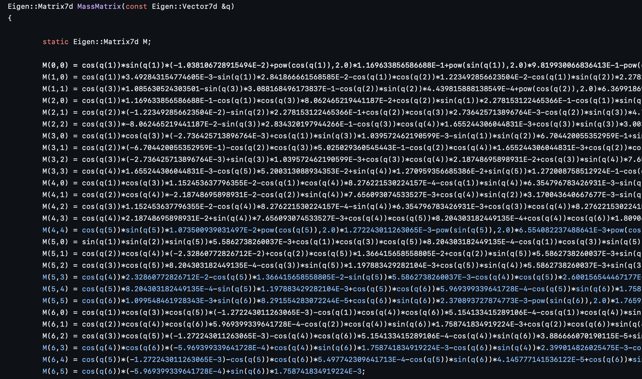
The aim of this project is to bypass the need for an explicit symbolic articulation of the EoM by formulating a neural network representation. With an accurately modeled neural network, it could serve as a foundational element in the development of an adaptive controller. The goal is for the controller to adapt a robotic arm’s physical parameters based on calibration sequences and to estimate the mass and inertia matrix of unfamiliar payloads.
Aside from symbolic representation, the EoM can also be computed numerically at each operating point using the Recursive Inertia Matrix Method
Background and Related Work
Before we delve into neural net architecture, let’s take a look closer at our problem and how it’s solved right now. To come up with the symbolic equation for the EOM, we use Lagrangian Mechanics in which we compute the Potential, U, and Kinectic Energy, T, of our system.
\(L = T - U\) \(\frac{d}{dt} \left( \frac{\partial L}{\partial \dot{q}_i} \right) - \frac{\partial L}{\partial q_i} = u_i\)
Quick describing of how it turns in into the manipulator equations. Working through these equations, a pattern emerge in which you can groups the equation as the manipulator equations.
\[M(q)q'' + C(q, q') = T(q) + Bu\]This method works well when the degree of freedom in the system is low. It provides much insight on how the dynamics of the system work. For example, the kinetic energy can be represented as:
\[T = \frac{1}{2} \dot{q}^T M(q) \dot{q}\]Highlighting that ( M ) is symmetric and positive definite. However, as introduced earlier, this method scales poorly with complexity in higher DOF systems.
However, as shown in the introduction, when this method is used for a 7 DOF system, the resulting equation is extraordinarily complex.
Bhatoo et al.
The other approach to create the manipulator equation is to numerically calculate it at each operating point. There are two versions of this equation, the inverse dynamics and the forward dynamics version. In the inverse dynamics formulation, we essentially calculate \(M(q)q'' + C(q, q') - T(q) = Bu\)
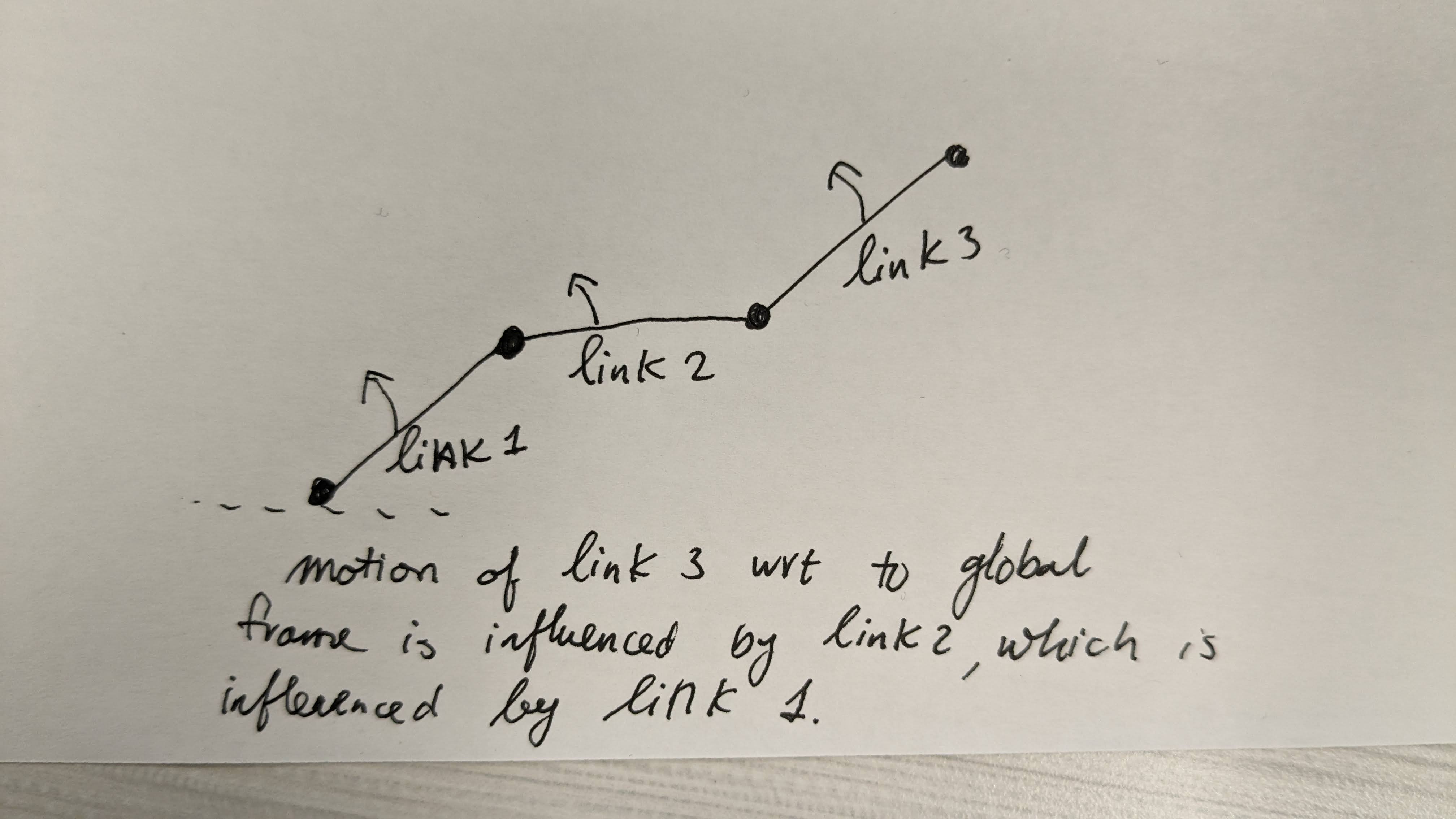
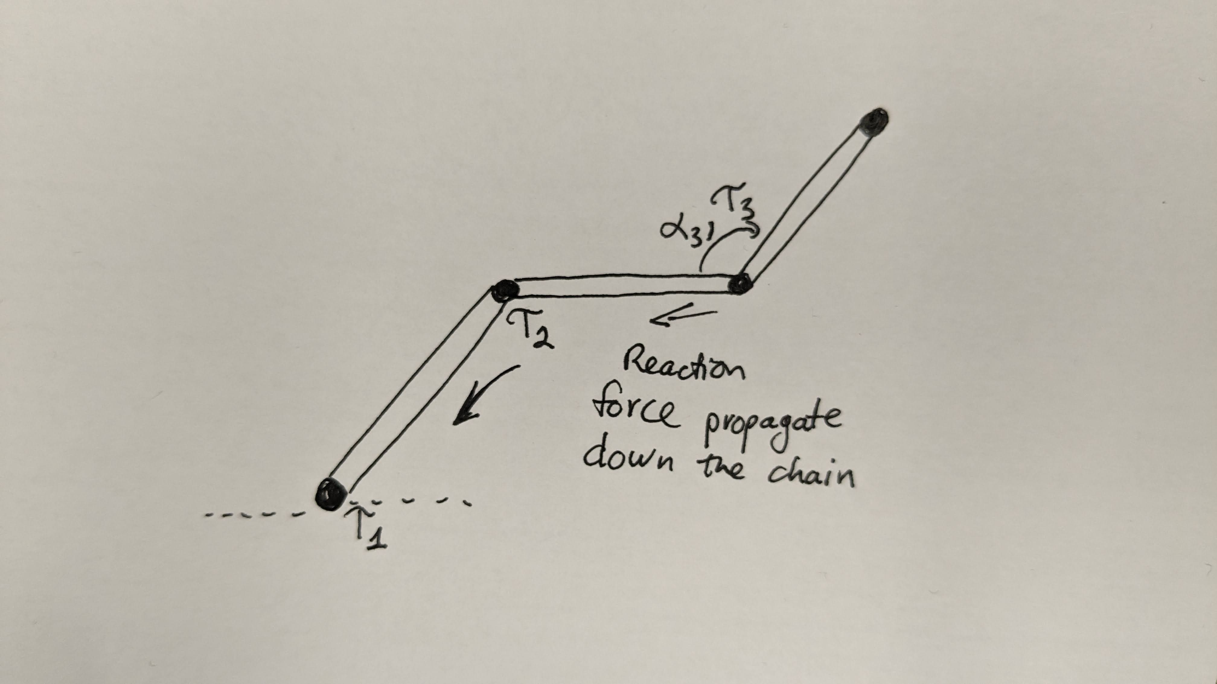
Giving a particular state of the robot and a desired acceleration, what is the required torque. The inverse dynamics formulation can be computed with the Recursive Newton-Euler Algorithm with a O(n) complexity where n is the number of joints
While very efficient to calculate, the inverse dynamics is not as useful as the forward dynamics version if the end goal is to create an adaptive controller. The forward dynamics is the model that describes what is the accelerations of the system based on current state and torque input.
\[q'' = M(q) \ (- C(q, q') + T(q) - Bu)\]This formulation is more useful for adaptive controller as we can compared predicted acceleration and actual acceleration. Use their difference as a loss and to compute the gradient from the model parameters. The problem with the forward dynamics problem is that it requires a O(n^3) computation for a serially linked robot arm (the mass matrix inversion must be done). The algorithm for Forward Dynamics is called Inertia Matrix Method
Experiments and Results
Generating Training Data
Utilizing numerical methods implemented in MATLAB, we generated a large volume of training data, spanning the full operational space of the robot arm. We based our robot arm model on realistic parameters from the publicly available data of the Emika Franka Panda, comprising a total of 10 links, seven revolute joints, and two fixed joints. After disregarding the base link, we have a model with 10 parameters for each link (mass, center of mass as a 1x3 vector, and the symmetric inertia matrix flattened into a 1x6 vector) and joint properties (angle, angular velocity, angular acceleration, and torque).
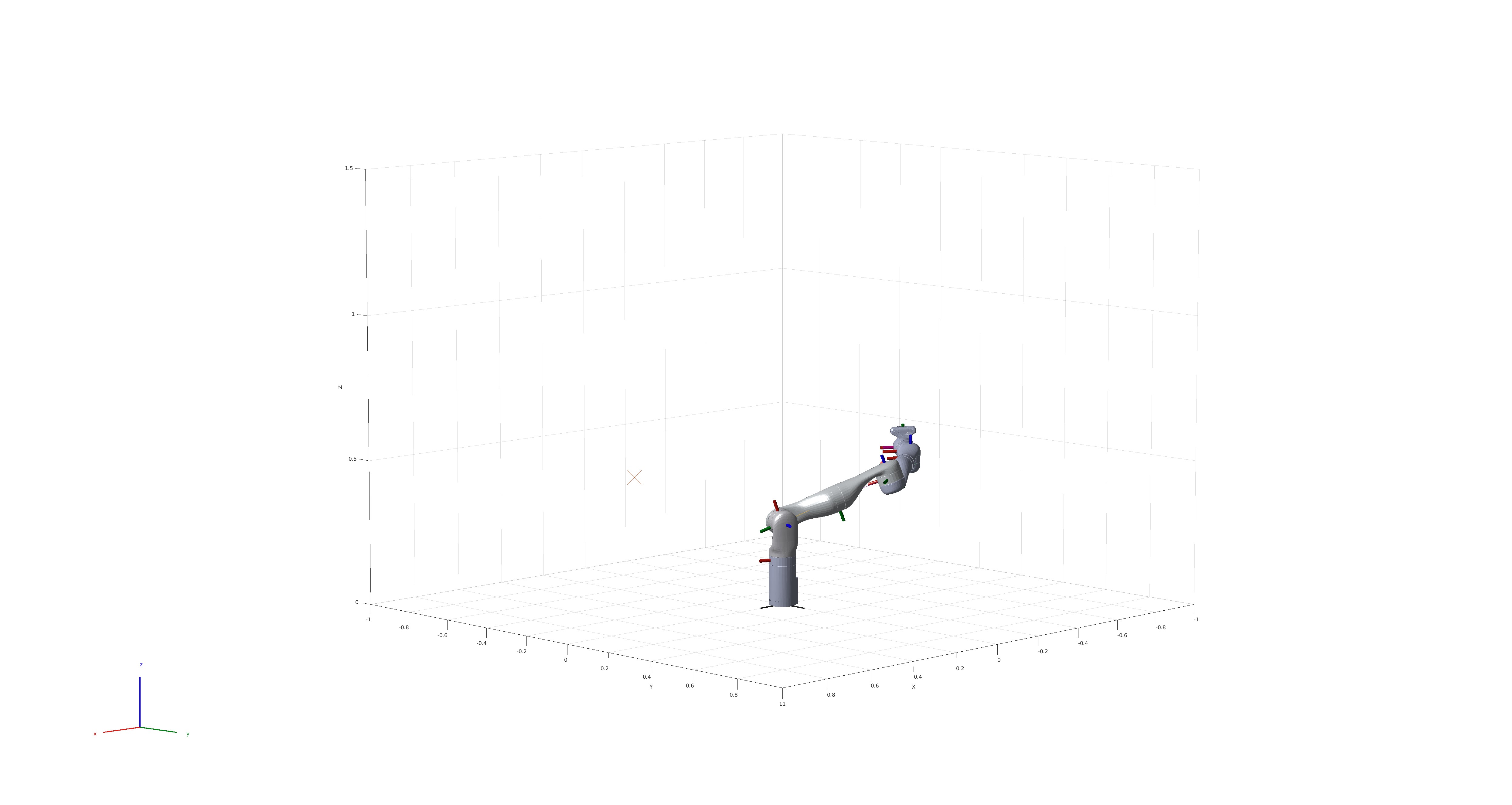
We simulated the arm moving from one random configuration to another—marked in the image above by an X — recording states, torques, and accelerations during transitions. To introduce variability, we applied realistic perturbations to the physical properties of each link after every 100 recorded motion paths. In total, we accumulated 250,000 data points
Attempt 1: Graph Neural Net
As inspired by Bhatoo, we rearrange the dataset as a Graph Dataset based on the PyTorch Geometric Library. Each node contains the 10 physical property parameters, angle, angular velocity, and torque input. In total, each node has 13 features. The output is set to be angular acceleration of the 7 joints (1x7 vector). As for the edge index, the graph is defined to be directed, either information flows from the last node to the first or the first node to the last node. This is inspired by the physical intuition that forces propagate sequentially from one body to the next, and that motion with respect to the global coordinate frame also sequential depended on the previous body link.
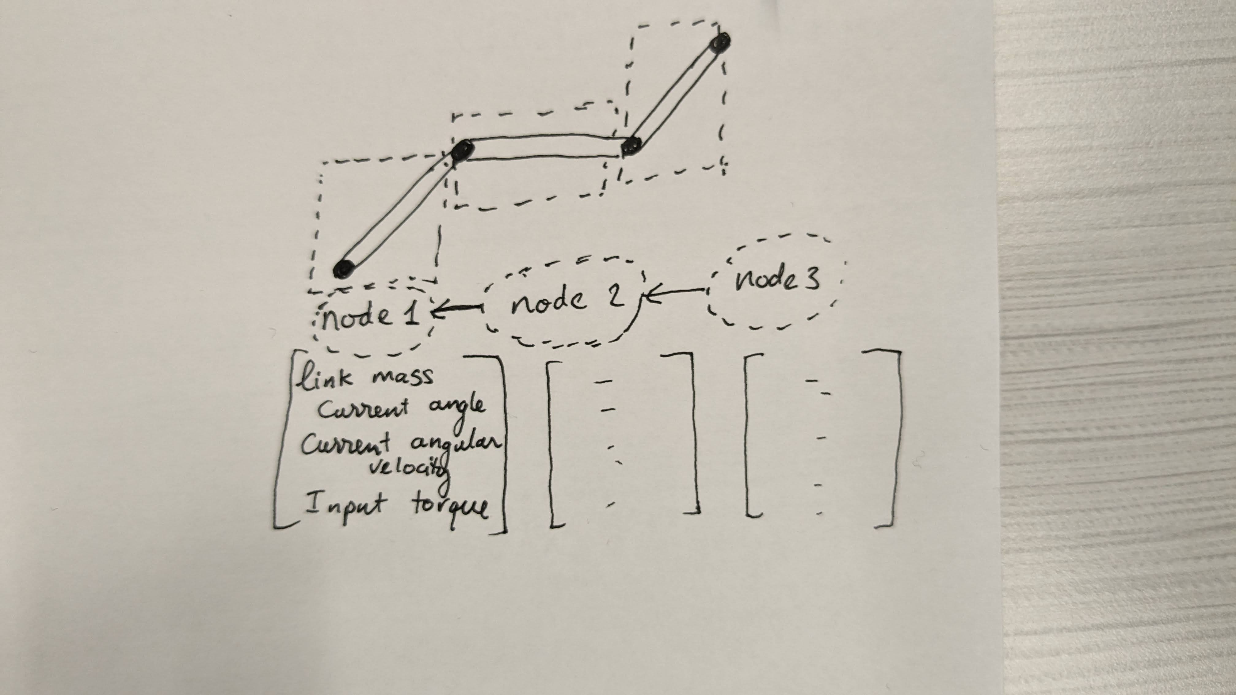
We applied nine iterations of the Graph Convolution Layer, ensuring information flow from one end of the arm to the other.
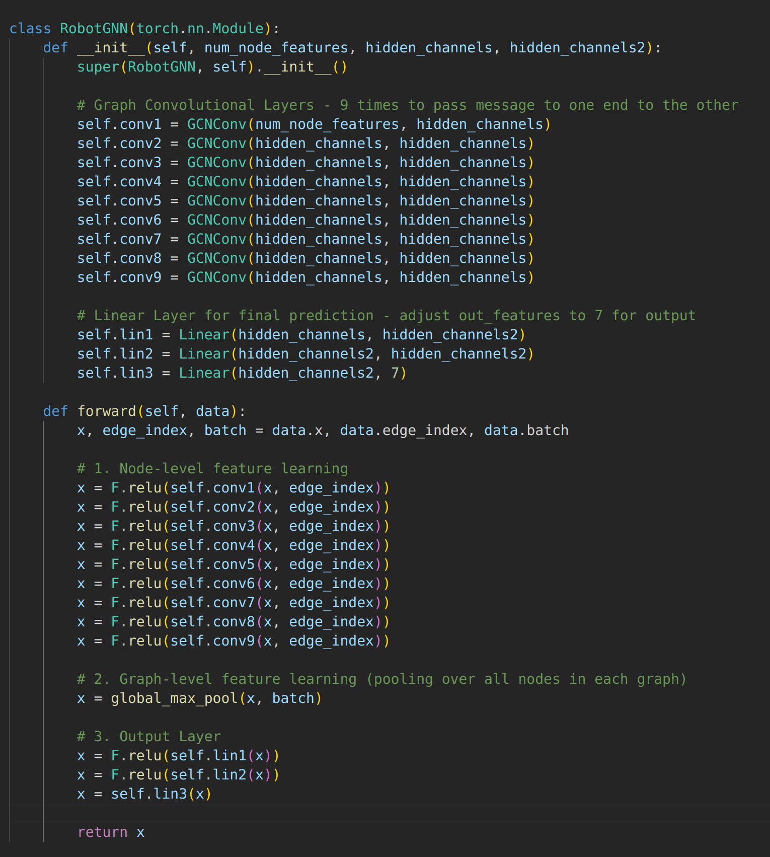
Despite extensive parameter tuning, learning rate adjustments, and the application of various schedulers, the loss showed no convergence. Potential reasons for this include the complexity in capturing temporal dependencies and the possible oversimplification of force propagation through the links using graph convolutions. The complexity of 9 different GCNV also increases complexity needlessly.

Attempt 2: LSTM
Reevaluating the necessity for graph neural networks, we considered the inherent sequential nature of the information flow in our system. There are no branches in the structure of a serially linked robot arm; hence, an LSTM, which excels in capturing long-range dependencies in sequence data, seemed appropriate. The input sequence now reflects the node properties from the previous attempt, and our LSTM architecture is defined as follows:
class RobotLSTM(nn.Module):
    def __init__(self, input_size, hidden_size, hidden_size2, output_size, num_layers=1):
        super(RobotLSTM, self).__init__()
        self.hidden_size = hidden_size
        self.num_layers = num_layers

        # LSTM Layer
        self.lstm = nn.LSTM(input_size, hidden_size, num_layers, batch_first=True)

        # Fully connected layers
        self.l1 = nn.Linear(hidden_size, hidden_size2)
        self.l2 = nn.Linear(hidden_size2, hidden_size2)
        self.l3 = nn.Linear(hidden_size2, output_size)

    def forward(self, x):
        # Initializing hidden state and cell state for LSTM
        h0 = torch.zeros(self.num_layers, x.size(0), self.hidden_size).to(x.device)
        c0 = torch.zeros(self.num_layers, x.size(0), self.hidden_size).to(x.device)

        # Forward propagate the LSTM
        out, _ = self.lstm(x, (h0, c0))

        # Pass the output of the last time step to the classifier
        out = out[:, -1, :]  # We are interested in the last timestep
        out = F.relu(self.l1(out))
        out = F.relu(self.l2(out))
        out = self.l3(out)

        return out
Despite the theoretically simpler representation of the system, the results were still not satisfactory, with stabilization and convergence being unachievable.

Attempt 3: Transformer
With LSTM and GNN strategies failing to deliver conclusive results, we pivoted to the more general-purpose Transformer architecture. This paradigm shifts focus from a strictly sequential data flow to a structure capable of interpreting the relationships between all links through its attention mechanism. Note, we also use a sinusoidal positional encoder to maintain the order coherance of the robot arm.
For the Transformer model, we employ the following architecture, designed to be flexible and adaptable to high DOF systems in future implementations:
class RobotTransformerModel(nn.Module):
    def __init__(self, input_dim=13, d_model=24, mlp_dim=128, nhead=2, num_encoder_layers=5, dim_feedforward=48, output_dim=7):
        super().__init__()
        self.d_model = d_model  # Store d_model as an instance attribute
        self.embedding = nn.Linear(input_dim, d_model)
        self.pos_encoder = PositionalEncoding(d_model) # Sinusoidal positional encoding
        # Transformer Encoder Layer
        self.transformer_encoder = Transformer(
            dim=d_model, mlp_dim=mlp_dim, attn_dim=dim_feedforward, num_heads=nhead, num_layers=num_encoder_layers
        )
        self.output_layer = nn.Sequential(nn.LayerNorm(d_model), nn.Linear(d_model, output_dim))
        self.criterion = nn.MSELoss()

    def forward(self, src):
        src = src.permute(1, 0, 2)  # Shape: [seq_len, batch, feature]
        src = self.embedding(src) * math.sqrt(self.d_model)
        src = self.pos_encoder(src)
        output, alphas = self.transformer_encoder(src, attn_mask=None, return_attn=False)
        output = output[0, :, :]  # use the output of the first token (similar to BERT's [CLS] token)
        return self.output_layer(output)
However, even with this advanced architecture, convergence remained elusive, indicating that further restructuring of the problem was required.

Final Attempt: Physics Informed Structured Transformer
As nothing seems to be working, we now simplify our problem statement to gain some insights that could then we applied to the larger problem later. First, we now reformulate the serially linked robot arm dynamics into a double pendulum system with simplified parameters—each link defined by its length and a point mass at the end. The state variables in this reduced complexity scenario are simply the two link angles and their angular velocities.
\[\mathbf{M}(q)\ddot{q} + \mathbf{C}(q, \dot{q})\dot{q} = \mathbf{T}_g(q) + \mathbf{B}u\]where
\[\mathbf{M} = \begin{bmatrix} (m_1 + m_2)l_1^2 + m_2l_2^2 + 2m_2l_1l_2\cos(q_1) & m_2l_2^2 + m_2l_1l_2\cos(q_2) \\ m_2l_2^2 + m_2l_1l_2\cos(q_2) & m_2l_2^2 \end{bmatrix},\] \[\mathbf{C} = \begin{bmatrix} 0 & -m_2l_1l_2(2\dot{q}_1 + \dot{q}_2)\sin(q_2) \\ \frac{1}{2}m_2l_1l_2(2\dot{q}_1 + \dot{q}_2)\sin(q_2) & -\frac{1}{2}m_2l_1l_2\dot{q}_1\sin(q_2) \end{bmatrix},\] \[\mathbf{T}_g = -g \begin{bmatrix} (m_1+m_2)l_1\sin(q_1) + m_2l_2\sin(q_1+q_2) \\ m_2l_2\sin(q_1+q_2) \end{bmatrix},\] \[\mathbf{B} = \begin{bmatrix} 1 & 0 \\ 0 & 1 \end{bmatrix}.\]In this simpler problem statement, we switch to solving the Inverse Dynamics problem instead which numerically has a computational complexity of O(n). We assume that there is less complexity in this representation (a complete guess), so the neural net doesn’t have to work as hard compared to the Forward Dynamics problem which has computational complexity of O(n^3).
However, the task now focuses on the inverse dynamics with a reduced computational complexity of ( O(n) ), given that ( M(q) ) can be linearly separated from ( C ) and ( T_g ) and knowing that ( M(q) ) is symmetric and positive definite.
For this, two Transformer neural networks were created, one for ( M(q)\ddot{q} ) and another for ( C(q, \dot{q})\dot{q} - T_g(q) ). Both models were trained separately with their respective datasets before being combined to model the complete manipulator equation. We can uniquely generate training data that only incite this mode by setting gravity and angular velocity to zero to get only M(q)*ddq = u.
The architectures for these Transformers were revised to employ a Physics Informed approach, ensuring the adherence to known physical laws:
class RobotTransformerModelH(pl.LightningModule):
    def __init__(self, input_dim = 3, d_model =3, mlp_dim=128, nhead=2, num_encoder_layers=5, dim_feedforward=48):
        super().__init__()
        self.d_model = d_model
        self.embedding = nn.Linear(input_dim, d_model)
        self.pos_encoder = PositionalEncoding(d_model)
        self.transformer_encoder = Transformer(dim=d_model, attn_dim=dim_feedforward, mlp_dim=mlp_dim, num_heads=nhead, num_layers=num_encoder_layers)
        self.output_layer = nn.Sequential(nn.LayerNorm(d_model), nn.Linear(d_model, 3))  # Output is a 1x3 vector
        self.criterion = nn.MSELoss()

    def forward(self, src, ddq):
        src = src.permute(1, 0, 2)  # Reshape for transformer
        src = self.embedding(src) * math.sqrt(self.d_model)
        src = self.pos_encoder(src)
        output, alphas = self.transformer_encoder(src, attn_mask=None, return_attn=False)
        output = output[0, :, :]
        output = self.output_layer(output)

        # Create a batch of symmetric 2x2 matrices from the batch of 1x3 output vectors
        batch_size = output.shape[0]
        symmetric_matrices = torch.zeros((batch_size, 2, 2), device=self.device)
        symmetric_matrices[:, 0, 0] = output[:, 0]
        symmetric_matrices[:, 1, 1] = output[:, 1]
        symmetric_matrices[:, 0, 1] = symmetric_matrices[:, 1, 0] = output[:, 2]

        transformed_ddq = torch.matmul(symmetric_matrices, ddq.unsqueeze(-1)).squeeze(-1)

        return transformed_ddq

Then we create a separate transformer neural net for C(q, dq)*dq - Tg(q). Similarly, we can generate training data that only exictes this mode by setting ddq = 0.
class RobotTransformerModelC(pl.LightningModule):
    def __init__(self, input_dim = 4, d_model =3, mlp_dim=128, nhead=2, num_encoder_layers=5, dim_feedforward=48):
        super().__init__()
        self.d_model = d_model
        self.embedding = nn.Linear(input_dim, d_model)
        self.pos_encoder = PositionalEncoding(d_model)
        self.transformer_encoder = Transformer(dim=d_model, attn_dim=dim_feedforward, mlp_dim=mlp_dim, num_heads=nhead, num_layers=num_encoder_layers)
        self.output_layer = nn.Sequential(nn.LayerNorm(d_model), nn.Linear(d_model, 2))  # Output is a 1x2 vector
        self.criterion = nn.MSELoss()

    def forward(self, src):
        src = src.permute(1, 0, 2)  # Reshape for transformer
        src = self.embedding(src) * math.sqrt(self.d_model)
        src = self.pos_encoder(src)
        output, alphas = self.transformer_encoder(src, attn_mask=None, return_attn=False)
        output = output[0, :, :]
        output = self.output_layer(output)

        return output

We picked Transformer as it’s more general compared to LSTM or GNN. Furthermore, it can easily be extended to high DOF system later on by just working with a longer input sequence. After training these two models independtly with their own training data set, we combined the two pretrained model togeher to recreate the full manipulator equation with a complete dataset.
lass CombinedRobotTransformerModel(pl.LightningModule): def init(self, config_H, config_C): super().init() # Initialize the two models self.model_H = RobotTransformerModelH(config_H) self.model_C = RobotTransformerModelC(config_C) self.criterion = nn.MSELoss() # Additional layers or attributes can be added here if needed
def load_pretrained_weights(self, path_H, path_C):
    # Load the pre-trained weights into each model
    self.model_H.load_state_dict(torch.load(path_H))
    self.model_C.load_state_dict(torch.load(path_C))

def forward(self, src_H, ddq, src_C):
    # Forward pass for each model
    output_H = self.model_H(src_H, ddq)
    output_C = self.model_C(src_C)
    # Combine the outputs from both models
    combined_output = output_H + output_C
    return combined_output
This modular approach, informed by the physical structure of the dynamics, resulted in improved convergence and an adaptive controller with the capability to generalize well to unseen conditions of the double pendulum.

Conclusion
Through this journey of building and testing various neural network architectures to approximate the equations of motion for high-DOF robotic systems, it becomes evident that while cutting-edge machine learning tools hold promise, their effectiveness is tied to the physical realities of the problems they aim to solve. Success in neural net modeling involves really understanding the data and problem you are trying to solve. Here we managed to make a little head way in modeling the EOM of a 2 DOF system by mimicking the structure of the analytical solution.
For future work, we should take the success in the 2 DOF system and push it for higher DOF with more complex parameters. We can generate data that can isolate specific motion modes of the model that can be used to train sections of the neural net at a time. By then training all the modes independently, we can stitch together the whole structure for the whole dataset.