Exploring Frobenius and Spectral Normalization in MLPs and Residual networks

This blog post compares the effects of a spectral view on weight normalization to a frobenius view on weight normalization normalization using a novel algorithm developed by us. We use two network types at multiple sizes to compare the effects of these two methods on the singular values of the weight matrices, the rank of the weight matrices, and the accuracy of the models.

Relevance and Investigation

Weight normalization in deep learning is vital because it prevents weights from getting too large, thereby improving model’s learning ability, accelerating convergence, and preventing overfitting. One traditional method for weight normalization involves adding the sum of the weights’ Frobenius norms to the loss function. One of the issues with penalizing Frobenius normalization of weight matrices is that it imposes a more strict constraint than may be desired for some model types- it enforces that the sum of the singular values is one, which can lead to weight matrices of rank one, which essentially enforces models to make decisions based on only one feature. In 2018, Spectral normalization emerged as an effective method, especially for Generative Adversarial Networks (GANs), to control the Lipschitz constant of the model and stabilize the training process . Spectral normalization is a more relaxed form of weight normalization that scales weight matrices based on their spectral norms, which is the maximum singular value of the matrix. This method is more relaxed because it does not impose a constraint on the sum of singular values, but rather only on the maximum singular value. This allows for weight matrices of higher rank, which may be more desirable for certain model types. Since 2018, spectral normalization has been used in many GAN architectures, but has not been explored as much in other deep learning scenarios. In fact, there is little published research on other approaches to the spectral view of weight normalization in general.

We introduce two novel normalization techniques inspired by AdamW and motivated by issues caused by penalties in the loss function . Our method, which we call Norm Scaling, takes a training step using a loss function that does not include a norm penalty, then scales the norms of the weight matrices after the step. Comparing our Frobenius and spectral normalization algorithms to each other can provide valuable insights into their advantages and disadvantages in various model architectures through a thorough investigation of their effects on the weight matrices. We aim to understand how the spectral norm of weight matrices change over time and how they affect overall model performance. Furthermore, we want to see how singular values change across architectures and algorithms, determining if certain types of architectures can benefit more from spectral normalization than another. It especially becomes interesting to investigate whether spectral normalization’s superior performance in stabilizing GAN training is generalized to other deep learning scenarios via different architecture types and a different scaling technique. The ultimate goal of this exploration is to deepen our understanding of these normalization techniques to find more intelligent ways to regularize weight matrices in order to acheive less overfitting and improve learning ability.

Norm Scaling

Let us introduce our novel normalization technique, Norm Scaling. We will first describe the algorithm in the context of Frobenius normalization, then we will describe how it will be applied with spectral normalization. We begin each process by initializing the weight matrices of the model to be orthogonal, which helps prevent gradient numerical stability issues and improve convergence timing. We then multiply each weight matrix, \(W_k\) by \(\sqrt{\frac{d_k}{d_{k-1}}}\) where \(d_k\) is the size of the output at layer \(k\). This enforces the initial spectral norm of each weight matrix to be \(\sqrt{\frac{d_k}{d_{k-1}}}\), and the initial Frobenius Norm to be \(\sqrt{min(d_k, d_{k-1})*\frac{d_k}{d_{k-1}}}\).

In the Frobenius Norm Scaling algorithm training is relatively straightfoward. After we initialize the orthogonal weight matrices but before beginning training, we calculate the Frobenius norm of each weight matrix based on the equation above and save these in our model. On each training step, we first calculate the loss, compute the gradients, and take a step using the optimizer. Then, we calculate the Frobenius norm of each weight matrix, \(W_k\), divide the matrix by this norm, and multiply it by its initial value that we calculated before training:

\[\bar{W}_k = \frac{W_k}{||W_k||_F} * \sqrt{min(d_k, d_{k-1})*\frac{d_k}{d_{k-1}}}\]

This ensures that the Frobenius norm of each weight matrix, \(W_k\), is equal to its initial value throughout the entire training process.

The Spectral Norm Scaling algorithm is slightly more mathematically complicated, and required the use of power iteration to make sure training time was feasible. After we initialize the orthogonal weight matrices but before training, we save target spectral norms for each weight matrix, \(W_k\). On each training step, we first calculate the loss, compute the gradients, and take a step using the optimizer. Then, we calculate the first singular value, which is the same as the spectral norm, and the first right singular vector of each weight matrix, \(W_k\), using power iteration. In order to mimimize the difference beween the right singular vector and the power iteration prediction of this vector we use 500 steps. To use power iteration with convolution weight matrices, which have dimension 4, we view them as 2 dimension weight matrices where all dimensions past the first are flattened (this reshaping is the channel-wise decomposition method and was used for similar work in Yang et al., 2020 ).

To find the first right singular vector and singular value, we use the fact that the top eigenvector and corresponding eigenvalue of \(A^TA\) are the first right singular vector and singular value of A respectively. So using the power method, we compute the top eigenvector and eigenvalue of \(W_k^TW_K\). We then use the fact that \(W_kv_1 = \sigma_1u_1\) to compute \(u_1 = \frac{W_kv_1}{\sigma_1}\).

We then perform the following normalization step:

\[\bar{W}_k = W_k + u_1v_1^T(\sigma^* -\sigma_1)\]

Where \(\sigma^*\) is the target spectral norm described above.

Note that this calculation subtracts the best rank one approximation of \(W_k\) from \(W_k\), but adds the same outer product back, scaled by \(\sigma^*\). Note that this does NOT enforce that the new spectral norm is \(\sigma^*\), because it is possible that \(\sigma_2\) is greater than \(\sigma^*\). We hope that this normalization prevents the first outer product of singular vectors from dominating the properties of the weight matrix, thus allowing for better generalization outside of the training distribution.

Experiments

In order to test our Norm Scaling learning algorithm, we train a variety of models on image classification of the CIFAR100 dataset . We train two types of models, MLPs and ResNets . Our MLPs consist of fully connected layers without biases, where our medium MLP has 5 layers each with 2,000 hidden units and our large MLP has 7 layers each with 4,000 hidden units. Our ResNets are ResNet34 and ResNet50, loaded in without pre-training. We adjust the size of the first convolution layer to 64 channels of 3x3 kernels and the output layer to output 100 classes. We train each of these four models with three different conditions: the first uses no weight scaling, the second uses Frobenius norm scaling, and the third uses spectral norm scaling. We train each model for 200 epochs with a batch size of 512, an initial learning rate of 0.001, and no weight decay. We use the Adam optimizer and a multi-step learning rate scheduler with \(\gamma = 0.1\) applied at epochs 60 and 120. We use the cross entropy loss function for all models. We use the same training hyper-parameters for all models. The models were trained on 4 NVIDIA Tesla A100 GPUs with paralellization handled by the pytorch lightning library.

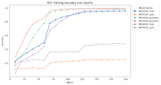
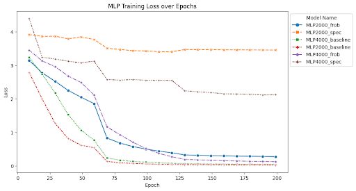
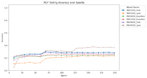
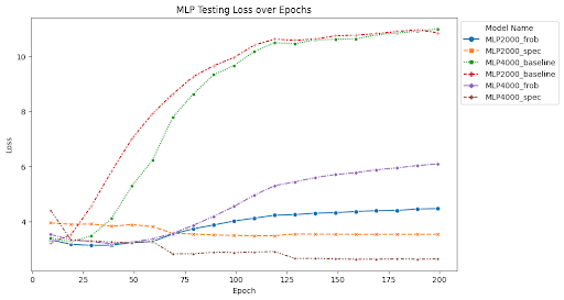
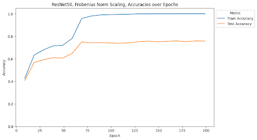
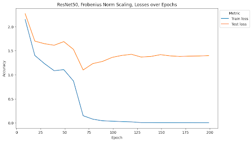
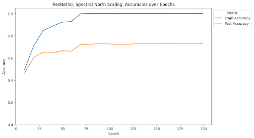
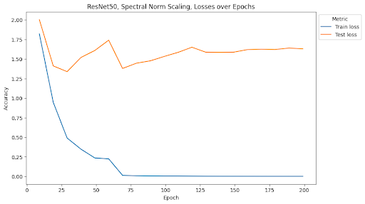
At the end of training, the MLP with depth 5, width 2000, and no norm scaling had a test accuracy of 25.12% and a test loss of 10.86. The MLP with depth 5, width 2000, and Frobenius norm scaling had a test accuracy of 28.23% and a test loss of 4.47. The MLP with depth 5, width 2000, and spectral norm scaling had a test accuracy of 23.21% and a test loss of 3.53. The MLP with depth 7, width 4000, and no norm scaling had a test accuracy of 23.95% and a test loss of 11.00. The MLP with depth 7, width 4000, and Frobenius norm scaling had a test accuracy of 26.62% and a test loss of 6.10. The MLP with depth 7, width 4000, and spectral norm scaling has a test accuracy of 36.25% and a test loss of 2.63. ResNet34 with no norm scaling had a test accuracy of 70.1% and a test loss of 2.03. ResNet34 with Frobenius norm scaling had a test accuracy of 75.24% and a test loss of 1.46. ResNet34 with spectral norm scaling had a test accuracy of 71.79% and a test loss of 1.78. ResNet50 with no norm scaling had a test accuracy of 73.45% and a test loss of 1.72. ResNet50 with Frobenius norm scaling had a test accuracy of 75.72% and a test loss of 1.40. ResNet50 with spectral norm scaling had a test accuracy of 73.29% and a test loss of 1.63. Full summaries of the changes of these metrics across epochs are plotted below with checkpoints every 10 epochs.

Above left: Training accuracy of MLPs. Above right: Training loss of MLPs. Spec refers to models trained with spectral norm scaling, Frob refers to models trained with Frobenius norm scaling, and Baseline refers to models trained with no norm scaling.

Above left: Testing accuracy of MLPs. Above right: Testing loss of MLPs.

Above left: Training accuracy of ResNets. Above right: Training loss of ResNets.

Above left: Testing accuracy of ResNets. Above right: Testing loss of ResNets.

Findings

Scaling Effects on Training Stability

One of the most interesting findings of this investigation is the effect of spectral norm scaling on the stability of training. We can see in the figures above that spectral norm scaling has a significant effect on the stability of training for MLPs, but not for ResNets. For MLPs, spectral norm scaling significantly improves the stability of training, as shown by the fact that the training and test loss curves remain close and follow a similar path. This is especially true for the large MLP, where the training and testing loss and accuracy curves maintain a similar relationship for the entire duration of training while the test loss increases and test accuracy plateaus for the other two normalization methods.

Above left: Testing and training accuracy of Large MLP (depth 7, width 4000) with no norm scaling. Above right: Testing and training loss, same model.

Above left: Testing and training accuracy of Large MLP with Frobenius norm scaling. Above right: Testing and training loss, same model.

Above left: Testing and training accuracy of Large MLP with spectral norm scaling. Above right: Testing and training loss, same model.

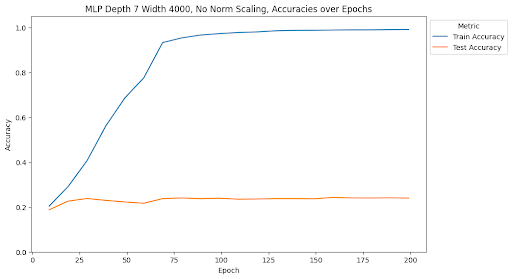
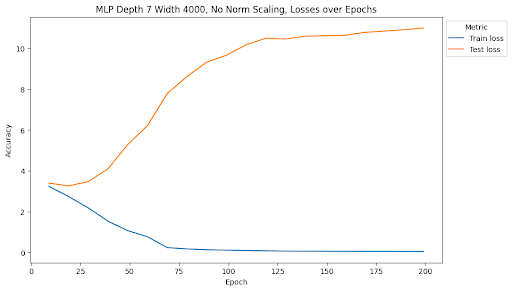
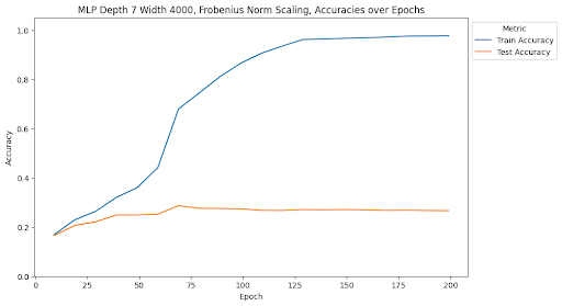
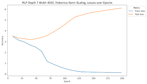
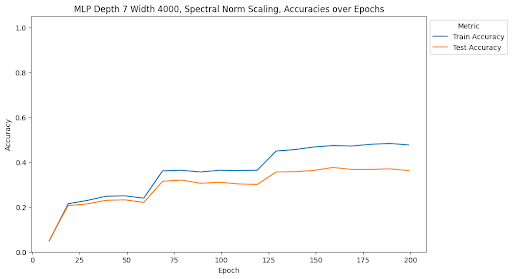
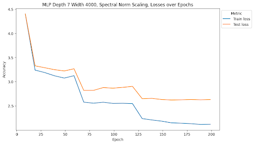
Although the train accuracy when using spectral norm scaling doesn’t get as high as in the other two models, it is an accuracy predictor for test accuracy during the entire training time. Furthermore, it is the only of the methods we tests that continues to decrease test loss for the duration of training, where the other two show signatures of overfitting the data and increasing test loss. This is a very interesting finding because it shows that spectral norm scaling can be used to improve the stability of training for MLPs, which is a very important property for deep learning models. This is especially true for MLPs because they are more prone to overfitting than other model types, so improving the stability of training can help prevent overfitting.

We see that this pattern does not hold for ResNets. Rather, it seems that the Frobenius norm scaling method introduces the most stability, but is still not stable as the relationship for spectral norm scaling in MLPs. Similarly, because ResNets rely on convolutions, we do not see issues with overfitting in any of the models. Altough it appears that spectral norm scaling may improve over the baseline stability, the effect is not as noticeable as the effect from Frobenius norm scaling.

Above left: Testing and training accuracy of ResNet50 with no norm scaling. Above right: Testing and training loss, same model.

Above left: Testing and training accuracy of ResNet50 with Frobenius norm scaling. Above right: Testing and training loss, same model.

Above left: Testing and training accuracy of ResNet50 with spectral norm scaling. Above right: Testing and training loss, same model.

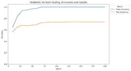
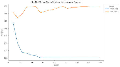
This is a surprising result considering that spectral normalization was first developed in the context of GANs using convolutional layers for image generation. We will address this disparity in the conclusion.

Scaling Effects on Spectral Norms

While both our spectral norm and Frobenius norm scaling algorithms resulted in consistently lower spectral norm values across all epochs compared to no normalization, spectral norm scaling had far and away the largest effect on enforcing low spectral norm values for weight matrices:

Changes in spectral norm values for each weight matrix in medium MLP (depth 5, width 2000) across epochs. Above left: No norm scaling. Above center: Frobenius norm scaling. Above right: Spectral norm scaling.

Changes in spectral norm values for each weight matrix in ResNet34 across epochs. Darker lines correspond to earlier layers. Above left: No norm scaling. Above center: Frobenius norm scaling. Above right: Spectral norm scaling.

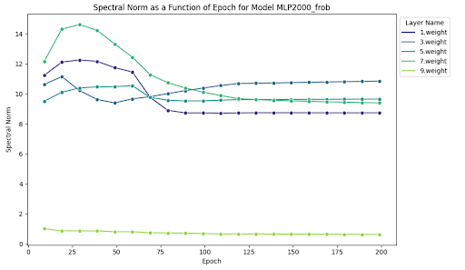
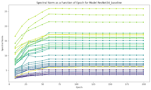
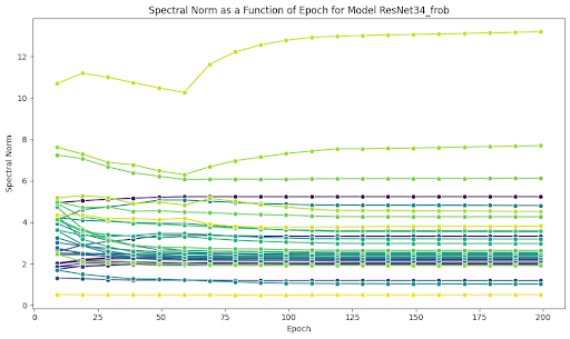
Using spectral norm scaling, the spectral norms of both architectures on all layers collapse to values significantly lower than those seen when using Frobenius norm scaling or no norm scaling. The average spectral norm values at the penultimate epoch (199) using spectral norm scaling is 0.8; Frobenius norm scaling is 7.8; and no normalization is 35.4 on the width 2000, depth 5 MLP architecture.

It is also interesting that spectral norms are very similar across layers in later epochs when using spectral norm scaling, but the same is not true for the other two experiments: the average standard deviation in spectral norm values across all layers for the last 100 epochs using spectral norm scaling is ~0.02; Frobenius norm scaling is ~3.7; and no normalization is ~18.4 on the width 2000, depth 5 MLP architecture.

While it may seem obvious that spectral norm scaling would do the best job at encouraging low spectral norm values, this was not evidently the case. While we subtract the best rank one approximation, thus decreasing the spectral norm, the new spectral norm does not necessarily become the target value, as it is possible that the second largest singular value is larger than our target spectral norm. It seemed possible that merely subtracting a rank one matrix would fail to completely curb spectral norm blow up or do it with this level of success. These results show that not only does our method do it successfully, but does it much more so than Frobenius norm scaling. What’s more, the results generalize across wildly different architectures: we see rapid convergence to low singular values in both the ResNet and MLP case roughly around the same epoch.

Conclusion

One drawback of our method was the significant increase in training times of our models. Compared to the time it took to train the baseline and Frobenius norm scaling implementations, the spectral norm implementations took between ~400% to ~1,500% longer to train. In order to address this in the future we will implement an adaptive power iteration that stops once the singular vectors converge to a certain threshold. This will allow us to reduce the number of power iterations needed to calculate the singular values, thus reducing the training time.

An interesting fold in our results was the difference between stability effects in the MLP and ResNet cases. We see that spectral norm scaling has a significant effect on the stability of training for MLPs, but not for ResNets. This is a surprising result considering that spectral normalization was first developed in the context of convolutional layers for image generation. We believe that this may stem from one of two reasons. The first is that we had to reduce the dimensionality of the convolutional matrices in order to use the power iteration algorithm. Although this allowed us to efficiently calculate the values we needed, it may not have been an accurate reflection of the matrix singular vectors. One route to address this in the future is to try initializing the spectral norm target values based solely on the input and output channel sizes, rather than the full size of the inputs and outputs. The second reason is that the convolutional layers in ResNets are not as prone to overfitting as the fully connected layers in MLPs, so the stability effects of spectral norm scaling would not be as noticeable. However, we still see an effect of Frobenius norm scaling, so this may be a matter of mathematical properties of the convolutional layers that we have not yet explored.

We may see most desired effects on singular values in spectral norm scaling because subtracting the best rank one approximation of the weight matrix does not influence other singular values nor the outer products of their singular vectors. When we view the singular value decomposition as the sum of outer products of singular vectors scaled by singular values, we can see that we only regularize one term in this sum. This may prevent a single outer product from dominating the linear transformation, especially preventing overfitting in MLPs where overfitting tends to be an issue. This is not true of Frobenius normalization, as we scale the entire matrix.

Overall, our results show that spectral norm scaling is a very effective method for stabilizing training in MLPs and enforcing low spectral norm values in MLPs and ResNets. This shows that spectral norm scaling may be a feasible and generalizable method for stabilizing training in a variety of conditions beyond GANs. Furthermore, we were able to achieve this without the use of a penalty in the loss function, achieving the same effect as a penalty without the negative effects. This is especially important because penalties in the loss function can cause issues with convergence and numerical stability alongside enforcing low rank, which we avoid by using our Norm Scaling algorithm. We beleive our results show great potential for further rigorous qauntitative research on the spectral view of weight normalization. We hope that our Norm Scaling algorithm will be used as a baseline for investigating spectral normalization algorithms that are both computationally efficient and effective at stabilizing training alongside enforcing low spectral norm values.

All of our training code can be found in this GitHub Repository.

---