Alive Scene

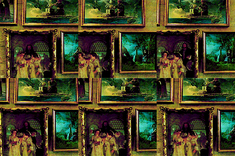
Inspired by the captivating Enchanted Portraits of the Harry Potter universe, my project unveils an innovative AI pipeline that transcends traditional scene-capture methods. Rather than merely recording scenes as a sequence of static images, this pipeline is intricately designed to interpret and articulate the dynamic behavior of various elements within a scene by utilizing CLIP semantic embeddings. This nuanced understanding enables the scenes to evolve autonomously and organically, mirroring the fluidity and spontaneity of living entities.

Enchanting Images with Semantic Embedding

“Alive Scene” is an advanced AI-driven project that revolutionizes the concept of scene capture, drawing inspiration from the enchanting, ever-changing portraits in the Harry Potter series. This innovative pipeline goes beyond traditional methods of capturing scenes as static images. Instead, it delves deep into the semantic understanding of each scene, enabling it to not only recreate these scenes with high fidelity but also to imbue them with the ability to act, evolve, and respond autonomously.

The following GIF image on the right is the output from the Alive Scene Pipeline. Notice that these scenes start from the same status.

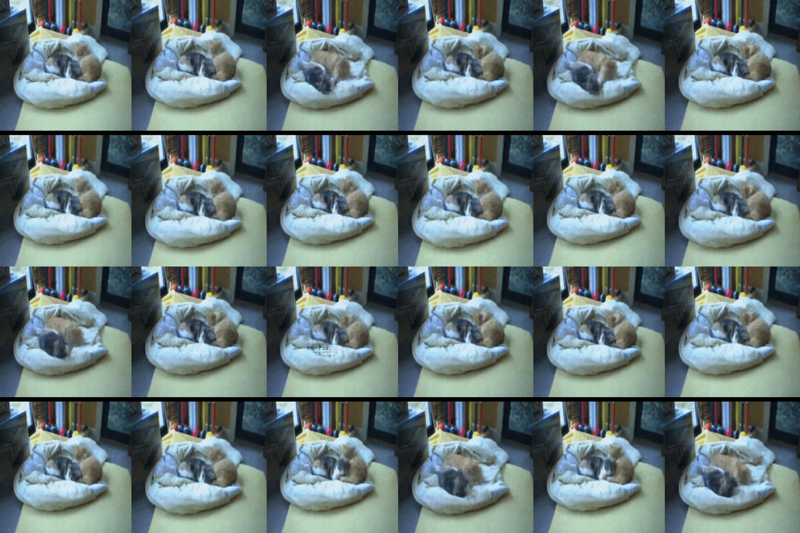
The core of this project lies in its sophisticated AI algorithms that analyze and interpret the nuances of each scene, from the physical elements to the underlying emotions and narratives. This enables the system to generate dynamic, lifelike representations that are far from static images. These AI-crafted scenes possess the unique ability to change organically over time, reflecting the natural progression and evolution one would expect in real life.

Through “Alive Scene,” portraits and scenes are no longer mere representations; they become entities with a semblance of life, capable of exhibiting behaviors and changes that mirror the fluidity and spontaneity of living beings. There are three elements in this project, the first is using CLIP model as encoder to compress image into clip embeddings. Second, train a generator to reconstruct the original image from the CLIP embedding. then train a behavior model to lean the behavior of clip embeddings in the clip feature space; the behavior will use to drive the generator; making the scene representation alive. The following is the diagrams of the pipeline.

Introduction

The CLIP (Contrastive Language–Image Pre-training) model, represents a groundbreaking approach in integrating visual and textual data within the realm of artificial intelligence. In this project, it plays and important role to comprehend the scenario and characters’ behaviors in the scene. Detailed investigations offers insightful understanding of the model’s operations, showing the potential that CLIP embeddings could make a machine comprehend and compress complex information of images.

The study explores using conditional Invertible Neural Networks (cINNs) for transforming still images into videos, highlighting cINNs’ prowess in handling static to dynamic content transitions. Although proficient in capturing motion, the model’s grasp on object/event types may benefit from CLIP embeddings enhancement. My project, unlike this work, aims to animate static scene representations with self-driven behaviors, not just manipulate videos.

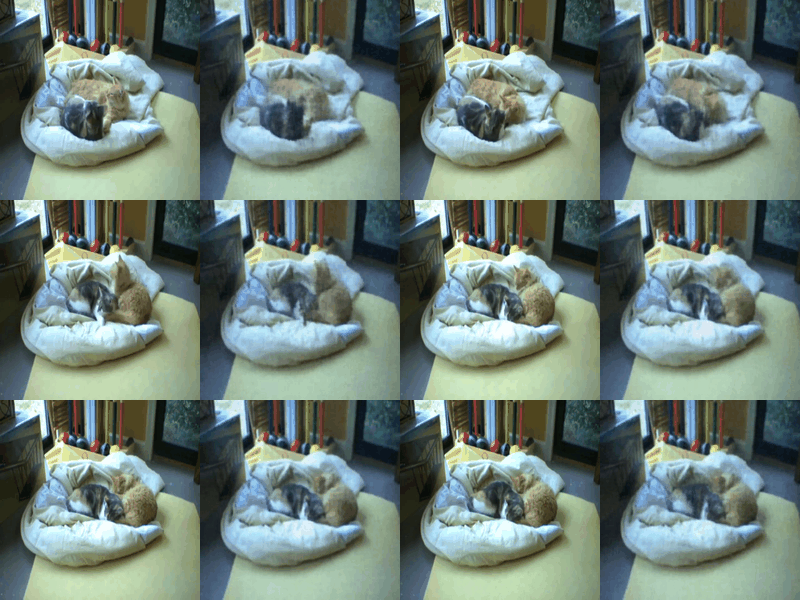
Another significant work, “Make-A-Video”, introduces a text-to-video generation method utilizing text-to-image models. This approach circumvents the need for text-video paired data, learning from text-image data and unsupervised videos. It employs a spatiotemporal diffusion model and super-resolution techniques for high-quality video creation from text. My project differs, focusing on bringing life to existing videos or image sequences, rather than generating new content from text.

Despite the static background, the cats’ movements are so subtle that they pose a challenge for human observers to distinguish differences between frames. To visualize the clip embeddings of the frames from the video, I employ both UMAP and t-SNE techniques for gaining more insights.

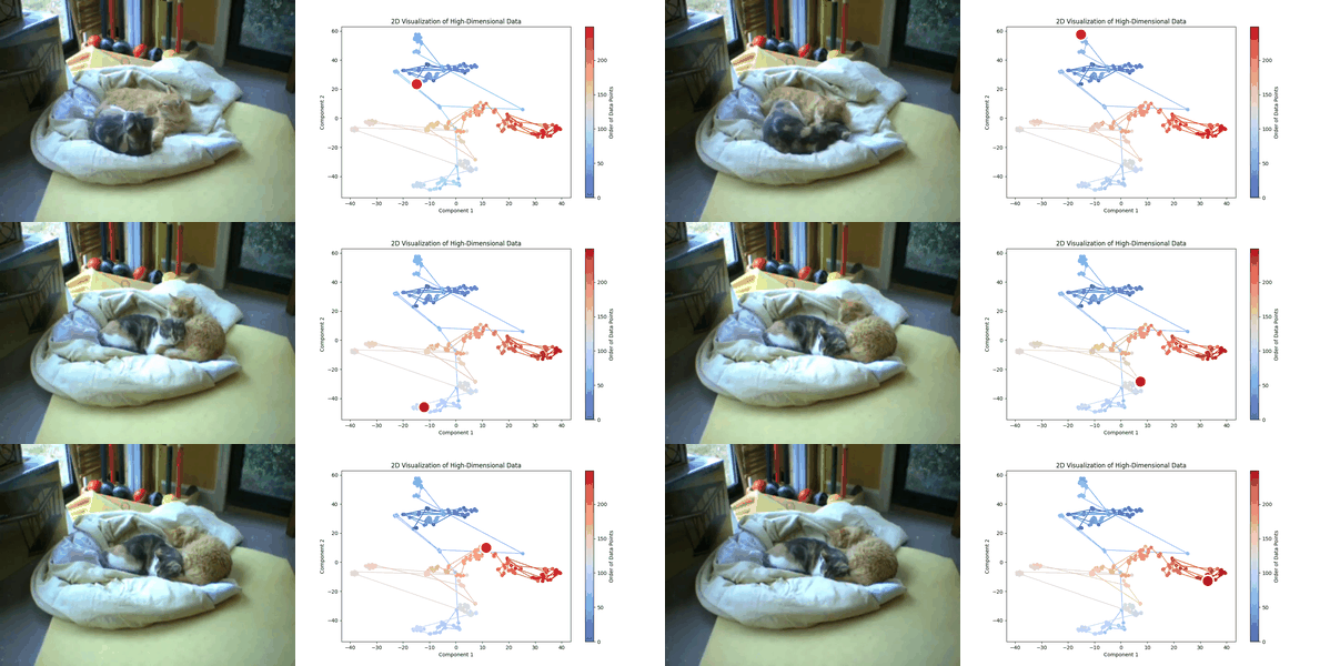
The behavior over time resembles a ‘spaghetti’ pattern, indicating that certain scenarios or behaviors may recur (as seen in the crossings or interactions within the spaghetti diagram). Some intersecting points demonstrate similar tendencies, while others are more unpredictable, highlighting the complexity of the video.

Both visualizations provide a promising sign: the end and start frames are positioned close to those in the middle. This proximity allows the Alive Scene to operate seamlessly and endlessly. For example, when the Alive Scene approaches a point near the end, it can smoothly transition to a frame somewhere in the middle. Similarly, when it encounters a region where different frames cluster together, it has a variety of options to choose from for its next move. This flexibility is key to making the Alive Scene function effectively.

Generator

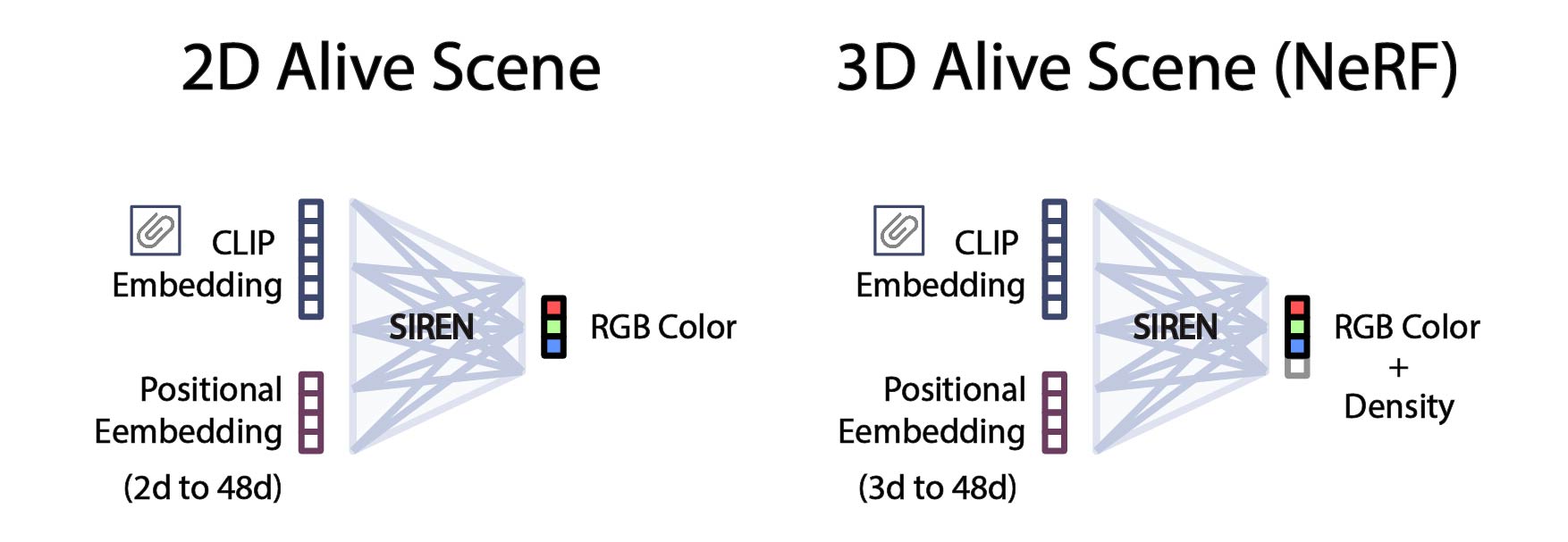
The Generator (decoder) is a SIREN model, which employs CLIP semantic embeddings and positional embeddings of pixel coordinates to generate RGB colors. SIRENs, or Sinusoidal Representation Networks, diverge from traditional neural networks by utilizing sinusoidal activation functions instead of common ones like ReLU. These networks are adept at implicitly representing intricate data patterns, making them particularly advantageous for tasks that involve complex spatial structures or continuous data. The incorporation of periodic activation functions in SIRENs can significantly enhance deep learning capabilities, especially in fields such as computer vision and generative models.

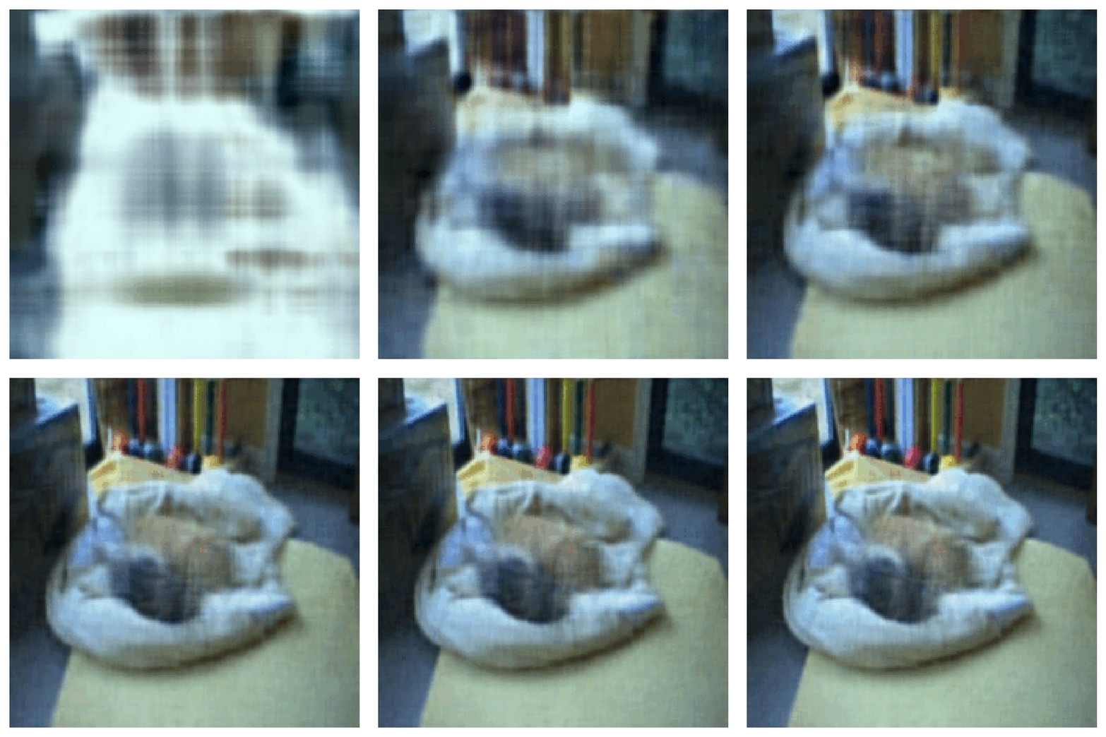
The code of the generator model (SIREN)

class SineLayer(nn.Module):

    def __init__(self, w0):
        super(SineLayer, self).__init__()
        self.w0 = w0

    def forward(self, x):
        return torch.sin(self.w0 * x)


class Siren(nn.Module):
    def __init__(self, w0=20, in_dim=560, hidden_dim=256, out_dim=3):
        super(Siren, self).__init__()

        self.net = nn.Sequential(nn.Linear(in_dim, hidden_dim), SineLayer(w0),
                                 nn.Linear(hidden_dim, hidden_dim), SineLayer(w0),
                                 nn.Linear(hidden_dim, hidden_dim), SineLayer(w0),
                                 nn.Linear(hidden_dim, hidden_dim), SineLayer(w0),
                                 nn.Linear(hidden_dim, out_dim))

        # Init weights
        with torch.no_grad():
            self.net[0].weight.uniform_(-1. / in_dim, 1. / in_dim)
            self.net[2].weight.uniform_(-np.sqrt(6. / hidden_dim) / w0,
                                        np.sqrt(6. / hidden_dim) / w0)
            self.net[4].weight.uniform_(-np.sqrt(6. / hidden_dim) / w0,
                                        np.sqrt(6. / hidden_dim) / w0)
            self.net[6].weight.uniform_(-np.sqrt(6. / hidden_dim) / w0,
                                        np.sqrt(6. / hidden_dim) / w0)
            self.net[8].weight.uniform_(-np.sqrt(6. / hidden_dim) / w0,
                                        np.sqrt(6. / hidden_dim) / w0)

    def forward(self, x):
        return self.net(x)


class MLP(nn.Module):
    def __init__(self, in_dim=2, hidden_dim=256, out_dim=1):
        super(MLP, self).__init__()

        self.net = nn.Sequential(nn.Linear(in_dim, hidden_dim), nn.ReLU(),
                                 nn.Linear(hidden_dim, hidden_dim), nn.ReLU(),
                                 nn.Linear(hidden_dim, hidden_dim), nn.ReLU(),
                                 nn.Linear(hidden_dim, hidden_dim), nn.ReLU(),
                                 nn.Linear(hidden_dim, out_dim))

    def forward(self, x):
        return self.net(x)


def train(model, model_optimizer, nb_epochs=15000):
    psnr = []
    for _ in tqdm(range(nb_epochs)):
        model_output = model(pixel_coordinates)
        loss = ((model_output - pixel_values) ** 2).mean()
        psnr.append(20 * np.log10(1.0 / np.sqrt(loss.item())))

        model_optimizer.zero_grad()
        loss.backward()
        model_optimizer.step()

    return psnr, model_output

Behavior model

This project introduces a customized asymmetrical Variational Autoencoder (VAE) as the probabilistic model to predict motion within the CLIP embedding space. A VAE-like model may prove beneficial for this task for two primary reasons. Firstly, they are adept at learning a continuous, smooth latent space, facilitating efficient interpolation and manipulation of data representations. Given that the training data derives from a video, it is inherently sequential and should be represented in a continuous fashion. Secondly, VAEs utilize amortized inference, where the encoder is trained to generalize the mapping of inputs to the latent space across the dataset, as opposed to conducting inference anew for each input. For this project, the objective is to devise a method that allows for a smooth navigation within the observed embedding space.

The code of the behavior model (VAE)

device = torch.device("cuda" if torch.cuda.is_available() else "cpu")
# BehaviorModel(inspired by VAE)
class BehaviorModel(nn.Module):
    def __init__(self, input_dim=512, latent_dim=256):
        super(VAE, self).__init__()

        # Encoder
        self.fc1 = nn.Linear(input_dim, 400)
        self.bn1 = nn.BatchNorm1d(400)
        self.fc2 = nn.Linear(400, 300)
        self.bn2 = nn.BatchNorm1d(300)
        self.fc21 = nn.Linear(300, latent_dim)  # Mean
        self.fc22 = nn.Linear(300, latent_dim)  # Log variance
        self.dropout = nn.Dropout(0.55)

        # Decoder
        self.fc3 = nn.Linear(latent_dim, 300)
        self.bn3 = nn.BatchNorm1d(300)
        self.fc4 = nn.Linear(300, 400)
        self.bn4 = nn.BatchNorm1d(400)
        self.fc5 = nn.Linear(400, input_dim)

    def encode(self, x):
        h1 = F.relu(self.bn1(self.fc1(x)))
        h2 = F.relu(self.bn2(self.fc2(h1)))
        h2 = self.dropout(h2)
        return self.fc21(h2), self.fc22(h2)

    def reparameterize(self, mu, logvar):
        std = torch.exp(0.5 * logvar)
        eps = torch.randn_like(std)
        return mu + eps * std

    def decode(self, z):
        h3 = F.relu(self.bn3(self.fc3(z)))
        h4 = F.relu(self.bn4(self.fc4(h3)))
        return F.tanh(self.fc5(h4))

    def forward(self, x):
        mu, logvar = self.encode(x.view(-1, 512))
        z = self.reparameterize(mu, logvar)
        return self.decode(z), mu, logvar

# Loss function
def loss_function(recon_x, x, mu, logvar):
    BCE = F.binary_cross_entropy(recon_x, x.view(-1, 512), reduction='sum')
    KLD = -0.5 * torch.sum(1 + logvar - mu.pow(2) - logvar.exp())
    return BCE + KLD

def loss_function(recon_x, x, mu, logvar):
    # Use Mean Squared Error for the reconstruction loss
    MSE = F.mse_loss(recon_x, x.view(-1, 512), reduction='sum')

    # KLD is unchanged
    KLD = -0.5 * torch.sum(1 + logvar - mu.pow(2) - logvar.exp())

    return MSE + KLD

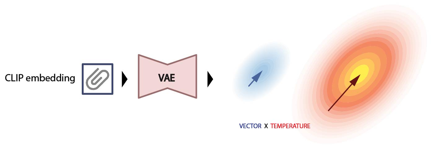
The process begins with a CLIP embedding as the input, which is then transformed by the model to output a motion vector. This vector retains the same dimensions as the CLIP embedding and is utilized to alter the original embedding, facilitating the generation of the subsequent frame based on this modified embedding.

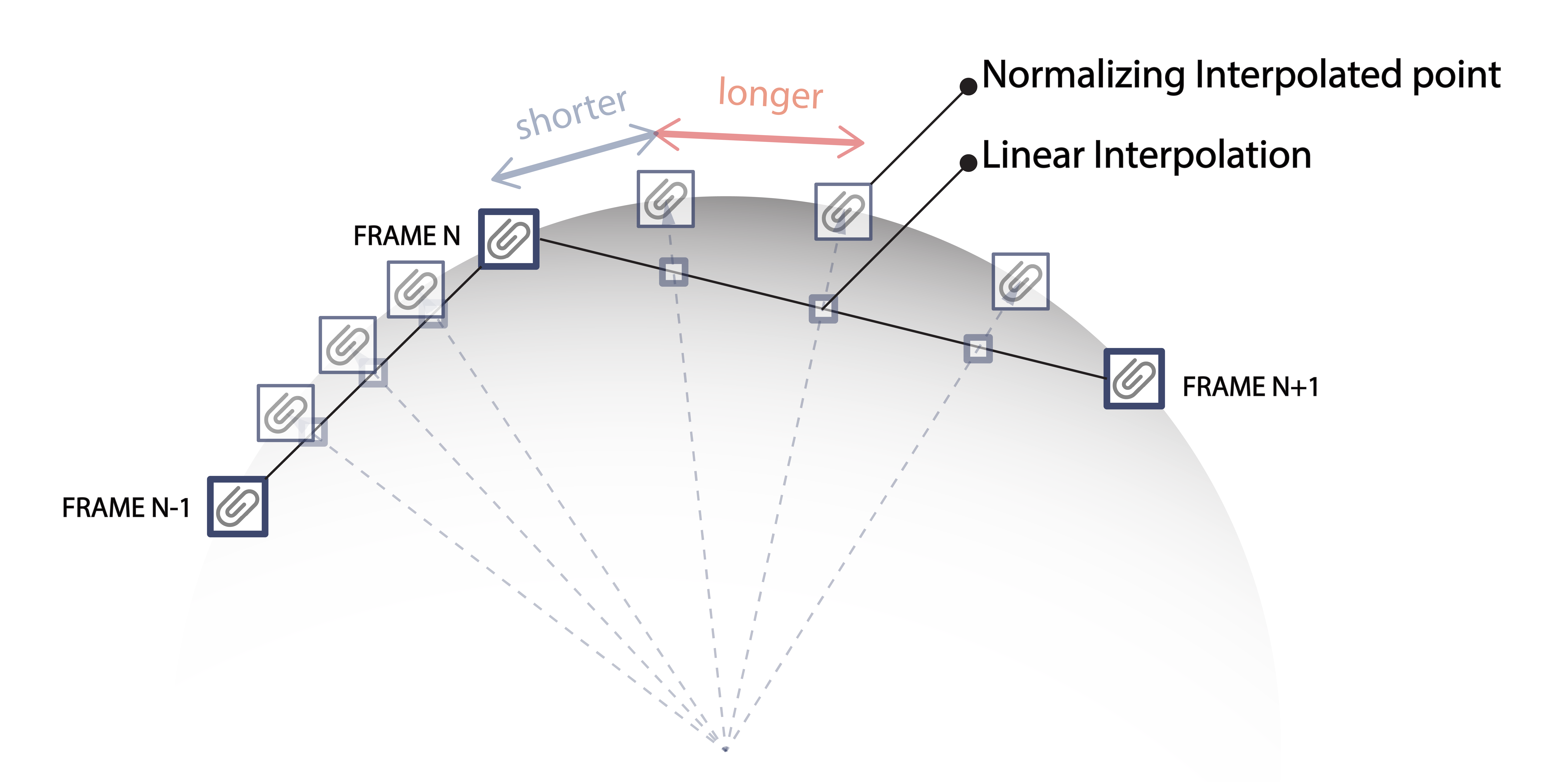
In this case, I generate 200 frames for training; the number is quite small. To enhance the model’s learning efficacy, new data points are generated through linear interpolation between existing data points (frames). By doing this, I generated 1000 clip embeddings and frames. These newly created samples undergo normalization to conform to the geometric constraints of the CLIP embedding space, often characterized as a hypersphere. This normalization process ensures that the interpolated data points adhere to the distribution pattern of the original embeddings. As depicted in the diagram, this technique leads to a densified clustering of data points in close proximity to the original embeddings, which is advantageous. It implies a higher confidence in the authenticity of these new points due to their closeness to the authentic, or ground truth, data.

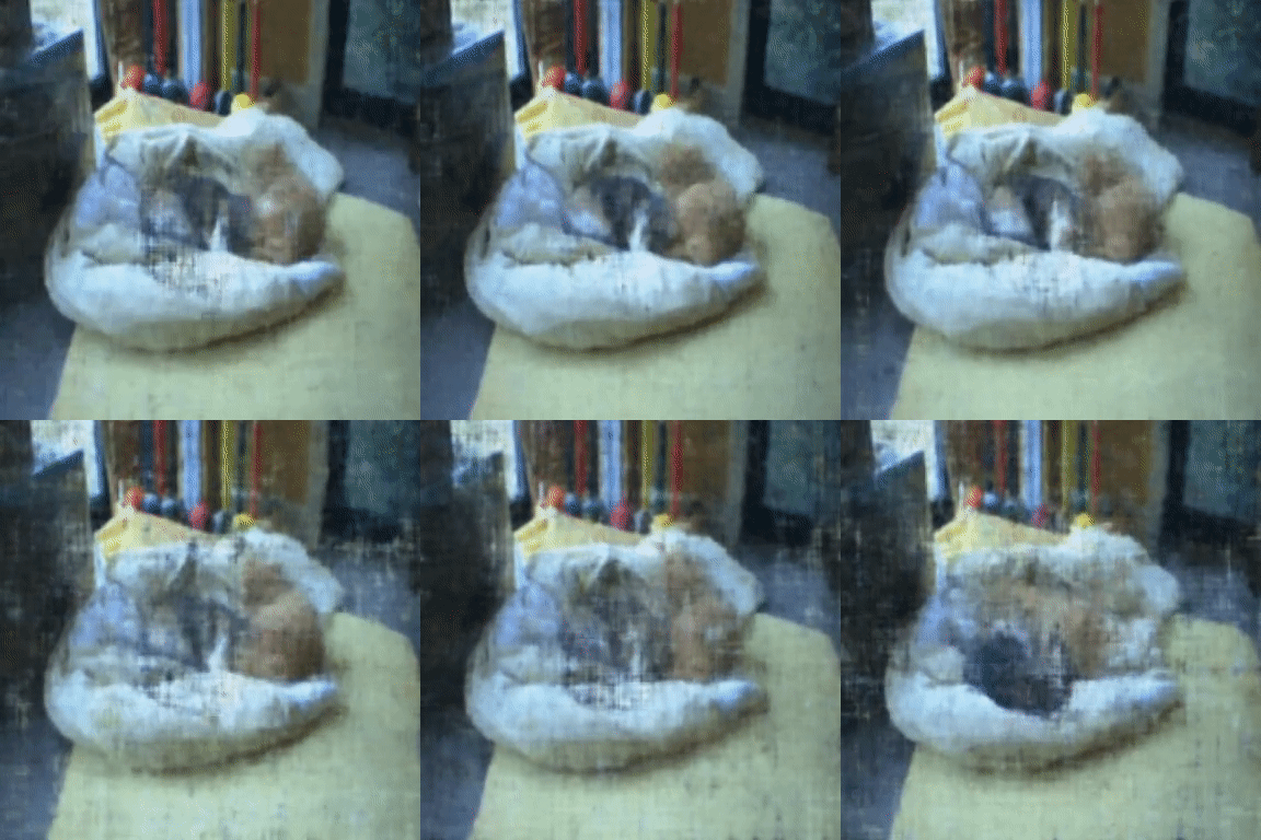
When operating the process that animates the Alive Scene, it occasionally generates artifacts. This may be caused by certain movements that deviate significantly from the observed reality. Please refer to the following GIF for an example.

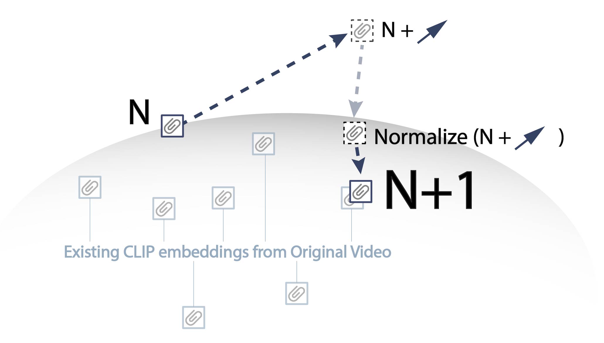
To resolve the issue, I have developed a post-processing technique that stabilizes the outcomes. The process begins by re-normalizing the resulting embedding onto the hypersphere. Following this, a weighted parameter is introduced to draw the vector incrementally toward the domain of previously observed CLIP embeddings. For example, if the weighting parameter is set to 0.1 for the observed embedding, it would be scaled by 0.1, while the predicted embedding is scaled by 0.9. These two are then summed to produce a final embedding that, while primarily influenced by the prediction, retains a subtle alignment with the observed data. This weighted approach aims to mitigate artifacts by anchoring the predictions within the realm of observed realities.

By applying this method, the Alive Scene has started to yield more stable results. Interestingly, the outcomes are varied, exhibiting behaviors akin to a living creature — somewhat unpredictable yet within a framework of predictability.

Manipulation

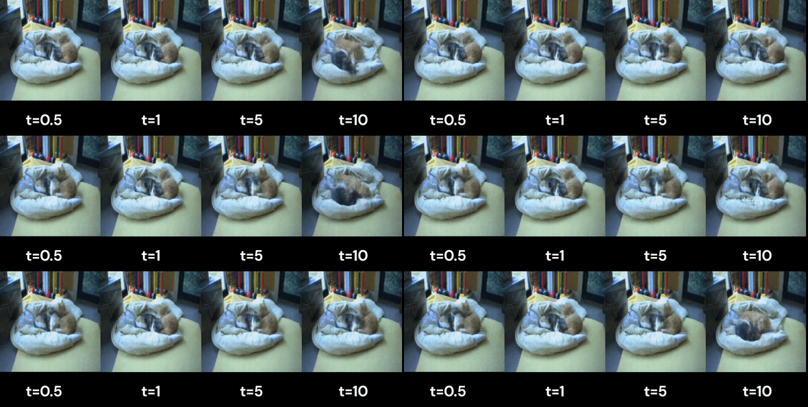
The Alive Scene operates autonomously, and to explore the modulation of its behavior, I have introduced the concept of ‘temperature.’ This concept acts as a coefficient that scales the movement vector, thereby allowing the scene to exhibit behaviors that are either more expansive and varied, or more constrained and subtle, depending on the temperature setting.

Conclusion

The “Alive Scene” project signifies a profound achievement in the domain of Deep Learning for scene representation. It leverages CLIP semantic embeddings to decode and imbue scenes with lifelike attributes, while also seamlessly integrating the potent SIREN model as a generator, capable of breathing vitality into the processed embeddings by producing authentic images.

Furthermore, the project implements an asymmetric Variational Autoencoder (VAE) to predict and model motion within the CLIP embedding space, thereby enhancing the dynamism and fluidity of the scenes.

However, the significance of this undertaking extends well beyond its technical accomplishments. By giving birth to scenes that autonomously and organically evolve, the project ushers in a transformative era of possibilities in digital storytelling and interactive media, fundamentally reshaping the landscape of creative expression in the digital realm.

Future Work

In this project, a SIREN model is trained to create a 2D scene representation. This model can be extended to generate a 3D scene by simply adding an additional output node to adopt the Neural Radiance Field (NeRF) architecture. Such an enhancement allows the 3D Alive Scene to offer a more immersive and complex scene representation. Looking ahead, it’s conceivable that a non-player character (NPC) could be manipulated in this manner, especially if the model, when trained on a vast dataset, can learn more sophisticated behaviors. This approach has the potential to encapsulate all necessary information within a highly compact model, offering an extremely lightweight solution for dynamic scene generation.

Potential Usages and Contributions:

Digital Art and Entertainment: This project can revolutionize digital art and entertainment by offering dynamic, evolving scenes that enhance animations and virtual experiences.

Film and Animation: It can automate the generation of realistic backgrounds, streamlining the production process for films and animated content.

Advertising and Marketing: The project offers the capability to create interactive, dynamic advertising content, thereby engaging audiences more effectively.

Behavioral Studies: It provides a tool for in-depth analysis of human and animal behaviors, supporting research in fields such as psychology, ethology, and anthropology.

Cultural Preservation: This technology can enliven historical scenes or artworks in museums, offering visitors more immersive and engaging experiences.

Data Visualization: It introduces innovative methods for interacting with and interpreting complex data, useful in sectors like finance and healthcare.

Gaming: The project enables the creation of NPCs with realistic behaviors, significantly enhancing the gaming experience.

Architecture and Engineering: It can be applied for dynamic visualizations in architectural and engineering projects, aiding in design and planning.

Conservation: This technology can contribute to wildlife conservation by facilitating the study of animal behaviors in natural settings.