Diffusion Models on Low-Brightness Images
Diffusion models have been used with great success for a number of use cases, but they still remain largely unused on dim images. The primary related work has been on using a diffusion model for low-light image enhancement. However, most of these works agree that attempting to generate an image from noise generated on top of an already dim image often results in rgb shift and global degradation of the image. This is because a diffusion model adds noise to the given image and then attempts to denoise the image, so given a dim and low-contrast image, the model has a difficult time denoising. This blog post focuses on methods to improve diffusion model performance in low-light images
Introduction
Since the introduction of ChatGPT, everyone seems to be speaking about “generative AI,” with almost 15x more google searches for generative AI now than at this time last year. This blog post focuses a specific use case for diffusion models, which have applications across the board, from generating images given keywords to planning trajectories for robot manipulation. In short, diffusion models are a family of probabilistic generative models that progressively destruct data by injecting noise, then learn to reverse this process for sample generation.
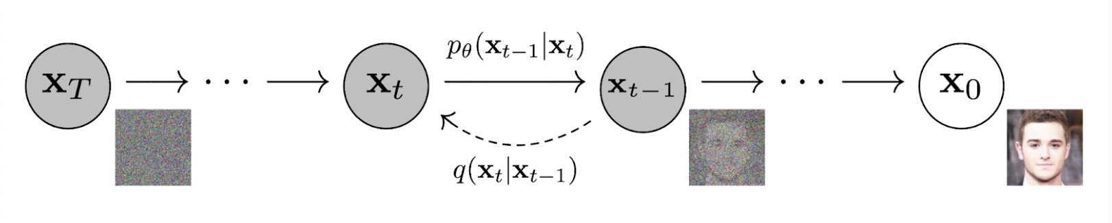 Figure 1.1. How a diffusion model iteratively transforms noise to generate an image
Diffusion models have been used with great success for a number of use cases, but they still remain largely unused on dim images. The primary related work has been on using a diffusion model for low-light image enhancement. However, most of these works agree that attempting to generate an image from noise generated on top of an already dim image often results in rgb shift and global degradation of the image
For a visual example of why low-light scenarios can be a problem for diffusion models, we can just look at the control of our experiments. The left image is from the diffusion model trained and evaluated on low-light images, while the right image is from the diffusion model trained and evaluated on normal-light images.
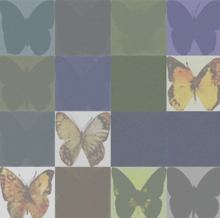
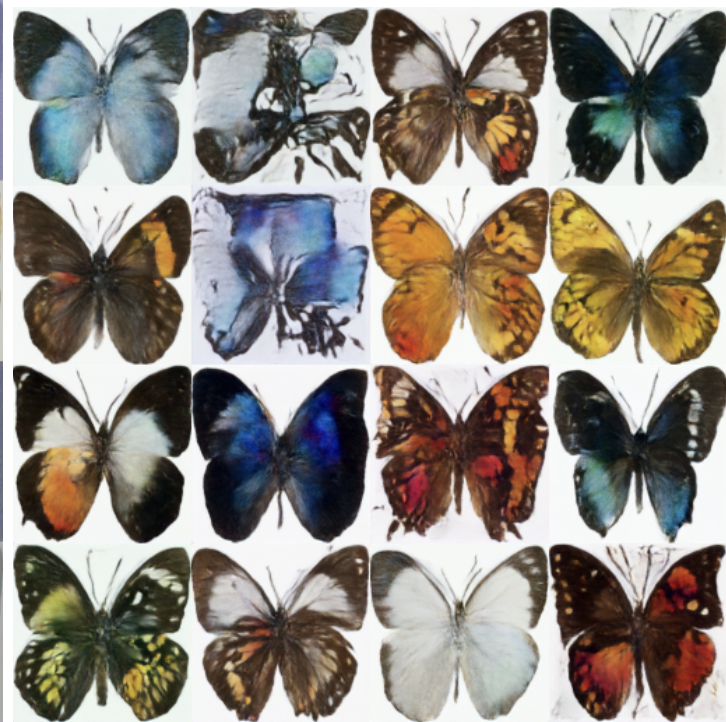
We can observe all sorts of problems here, from the model being unable to determine the image background color to the model sometimes not even showing the butterfly. In contrast, the exact same training done on the normal butterfly dataset shows distortions occasionally, but has no issues determining the background color or the contrast between the butterfly and the background. This illustrates the issue talked about previously of rgb shift and global degradation. In this blog, we aim to conduct experiments by adding different features to the DDPM scheduler and investigate which can actually make a difference for low-light scenarios.
Background
First, we discuss the idea of a diffusion model in more depth. In a nutshell, a diffusion model relies on semi-supervised training. The model is given an image from a training set to which random noise has been applied \(t\) times. This noisy image is given to the model along with the value of \(t\), a loss is computed between the output of the model and the noised image. The random noise is applied with a noise scheduler, which takes a batch of images from the training set, a batch of random noise, and the timesteps for each image. The overall training objective of the model is to be able to predict the noise added through the scheduler to retrieve the initial image.
Since diffusion models on dim images are relatively unstudied, this blog post focuses on taking a well-known diffusion model for regular images and making modifications to the scheduler, which controls the noising and denoising process, and the model architecture to improve its performance in low-light scenarios. We begin with the DDPM (Denoising Diffusion Probabilistic Models) model
A DDPM uses two Markov chains for its denoising and noising process: one to perturb the data to noise, and another one to convert the noise back into data
The specified beta values can have many consequences on the model overall, but one is more aggressive denoising which can combat rgb shift. This is because rgb shift can cause color inconsistencies between adjacent pixels, which can be combated by greater noise reduction. In addition, aggressive denoising may be able to recover the underlying structure of the image and smooth out artifacts introduced by rgb shift. However, aggressive denoising can result in a loss of detail as well
By integrating the previous noise during the noising step to determine \(q(x_T)\) we can get \(q(x_T) = \int q(x_T \vert x_0)q(x_0)dx_0 \sim \mathbb{N}(x_t; 0, I)\), showing that after all the noise is integrated, the entire structure of the image is lost. After the denoising, DDPMs start generating new samples by generating a noise vector from the prior distribution \(p(x_T = \mathbb{N}(x_T; 0, I)),\) and gradually removing noise by running a Markov chain in the reverse. The goal is to learn the transition kernel between timesteps. The reverse transition can be written as \(p_{\theta}(x_{t-1} \vert x_t) = \mathbb{N}(x_{t-1}; \mu_{\theta}(x_t, t), \sigma_{\theta}(x_t, t))\) where \(\theta\) is the model’s parameters and the mean and variance are parametrized by neural networks
This variance will also come into play later, as it is one of the parameters that we toggle in the DDPM scheduler. Variance in the DDPM Scheduler of the Diffuser library has several possible values: fixed_small, fixed_small_log, fixed_large, fixed_large_log
| variance_type | effect |
|---|---|
| “fixed_small” | The variance is a small and fixed value |
| “fixed_small_log” | The variance is small and fixed in the log space |
| “fixed_large” | The variance is a large and fixed value |
| “fixed_large_log” | The variance is large and fixed in the log space |
Methods
The first method evaluated as a control is simply an implementation of a DDPM using the Diffusers library
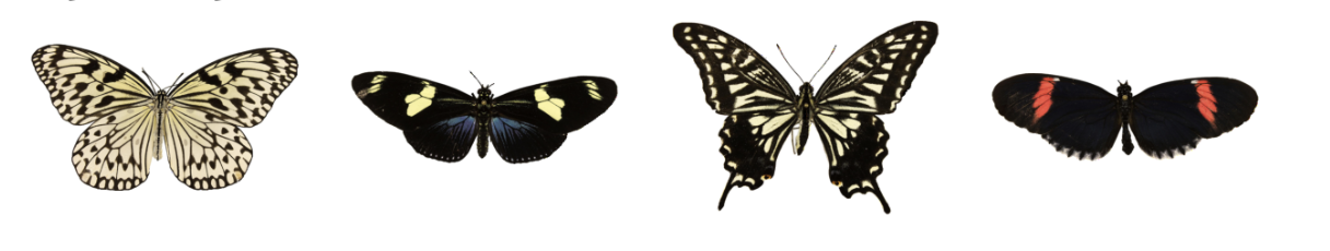
Figure 3.1. Original images from dataset
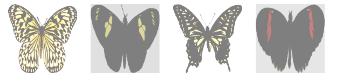
Figure 3.2. Images after preprocessing
Next, noise is added to the images. For this, we use the DDPMScheduler with the default parameters from Diffusers. The model is then trained on the noisy image, and evaluated. For evaluation, the model is tested on sixteen different images previously sampled randomly from the training dataset and set aside as test images. These images are noised using the scheduler in the same way as the rest of the images, and the model is run on the noised images to retrieve the original images.
| Control Parameters | |
|---|---|
| noise_timesteps | 50 |
| num_epochs | 50 |
| beta_start | 0.0001 |
| beta_max | 0.02 |
| variance_type | “fixed_large” |
| resnet layers per unet block | 2 |
Figure 4.1. Showing default parameters used in the diffusion model
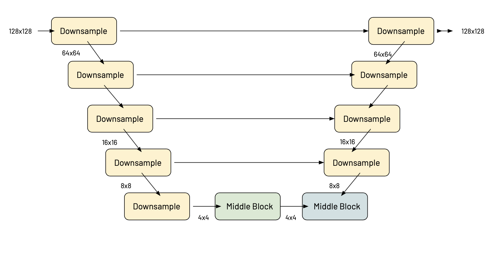 Figure 4.2. Figure depicting the UNet architecture used in the model
Initially, a quantitative method of evaluation was considered, and some losses were computed between the test images before noising and the corresponding test results after denoising. While these measurements were computed, they didn’t seem as valuable as simply looking at the image because of the various patterns between images that a loss function cannot always capture (ie how similar is the butterfly and the pattern of the butterfly to the initial image). As an example, the image on the left receives a lower mean squared error loss than the image on the right, yet looking at them, it is apparent that the denoised version on the right is better. Thus, the evaluation here mostly presents the model outputs for us to qualitatively compare across different variations.
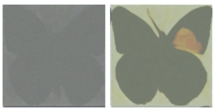 Figure 4.3. Showing two outputs of different models given the same input. MSE Loss proved to be unreliable for this task as the loss of the left image compared to the control was less than the loss of the right image due to rgb shift
After the control, this process is repeated for a variety of parameters carefully chosen and model architecture modifications to evaluate the best variation for use in this low-light scenario.
Results/Discussion
The results of the control are as seen in the introduction above. The result of the dim images is on the left, while the result of the brighter images is on the right.
Figure 5.1. The left shows the output of the control model trained on the dim images and the right shows it trained on the bright images
One of the most pressing problems seen on the dimmer images is the rgb shift. As discussed in the background, the variance, which partly controls how aggressively the model is denoised, can help with rgb shift because it larger denoising can retrieve details lost in noise. Thus, the first modification is changing the variance type from “fixed_small” to “fixed_large.” This modification, after training, resulted in the evaluation images below.
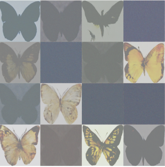
Figure 5.2. Result of evaluation after changing variance
As we can see, this helped greatly with the rgb shift issue, and eliminated the background discoloration for several of the images. Certain images, such as the second row on the left-most column and the third from the left on the bottom row also show huge detail improvements. For the reasons discussed earlier, this is expected as a result of larger denoising, since it can clear away ome artifacts. The only image that showed a decrease in quality after the variance change was the right-most image in the top row.
Now that some of the rgb shift has been resolved, we move to tackling the loss of detail in many of these evaluation images. One classic approach to loss of information is simply increasing the capacity of the model to learn. In more technical terms, by increasing the number of ResNet layers per UNet block, we may allow the model to capture more intricate features and details. Deeper layers can learn hierarchical representations, potentially improving the ability to encapsulate fine-grained information. To do this, we edit our model architecture to make each UNet block deeper.
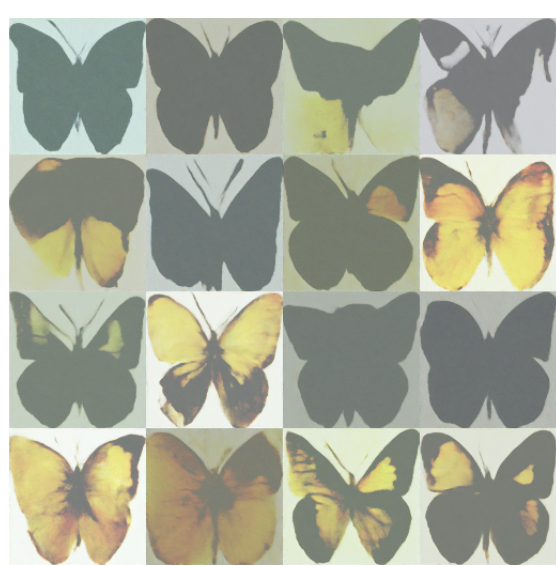 Figure 5.3. The left image shows the output of the new change in model architecture on the dimmed dataset, while the right image shows the bright dataset control output for color comparison
A huge improvement can be seen just by deepening the model architecture and at least the outline of every butterfly is now visible. However, this still hasn’t solved the problem of rgb shift. As we can see, the butterflies in the denoised dim images are all skewed yellow, while the butterflies in the denoised control bright images are all of varying colors. Next, we try to train with various betas in the scheduler to tackle this issue. As discussed before, higher beta values can help with rgb shift. However, higher values can also lead to loss of detail. The beta_start for the control was 0.0001 and the beta_max was 0.02. Thus, we try two combinations of start and max: 0.001 and 0.01, and 0.0005 and 0.015.
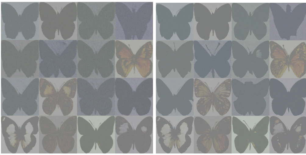
Figure 5.4. The left figure shows the output for beta start = 0.001 and beta end = 0.01, and the right figure shows the output for beta start = 0.0005 and beta end = 0.15
As seen above, this modification was unsuccessful, and the images have much less detail than before and the rgb shift is worse than before. This may be because the biggest issue is the distortion of colors and blurring, and thus, a high beta value and larger denoising is needed to fix these issues rather than smaller denoising as was previously hypothesized. This future modification is not analyzed in this project, but would be interesting to see in the future.
Future Directions
There are several limitations and future directions worth discussing. For one, this project investigates a specific model, the DDPM model. The DDPM model was chosen for various reasons, but mostly because it draws a balance between detail and also efficiency. In the future, multiple models could be considered to figure out which is really best for image generation under low-light scenarios. In addition, this work only focuses on one dataset of butterflies, and generates “low-light” data by reducing the brightness of the original dataset. This is good evidence for the success of the methods presented, but additional datasets and real data taken from environments with low-light would have lended more evidence to the success of the methods. In addition, the amount of data and depth of the models used had to be limited used to gpu usage limits. A model trained for more epochs with data may work better than this one. In addition, a good future starting point for this work would be to work with the beta start and beta max to figure out how to improve the rgb shift, which I believe would help with the detail in the dim images.