Investigating the Impact of Symmetric Optimization Algorithms on Learnability

Recent theoretical papers in machine learning have raised concerns about the impact of symmetric optimization algorithms on learnability, citing hardness results from theoretical computer science. This project aims to empirically investigate and validate these theoretical claims by designing and conducting experiments as understanding the role of optimization algorithms in the learning process is crucial for advancing the field of machine learning.

Introductions

Neural networks have been a staple in Deep Learning due to their expressive power. While the architecture itself is very powerful, the process of \textit{optimizing} the neural network - i.e., finding the values of the parameters of the network that minimize the loss over training data - is approximate. After all, a neural network is a highly non-smooth function and is inherently difficult to optimize. The core idea of many of these methods is to approximate the neural network (i.e. via first or second-order approximations), which are then easier to optimize over.

Our goal is to explore if incorporating “asymmetries” into optimization can help. Many methods use a similar update rule for all parameters in the network. We experiment with using different rules for different parameters, guided by heuristics.

Motivation: a couple of nice papers

This project is motivated by a couple results, not necessarily in the context of neural networks. The first comes from a 2004 paper by Andrew Ng titled “Feature Selection, $L_1$ vs. $L_2$ regularization, and rotational invariance”. It concerns the sample complexity of feature selection - how much training data is necessary to fit the model to some accuracy with high probability - where the number of relevant features is small compared to the total number of features. The paper shows that the mode of regularization is of utmost importance to the sample complexity: the sample complexity using $L_2$ regularization is exponential compared to the sample complexity with $L_1$ regularization. One may ask: what does this have to do with symmetry? In the case of $L_2$ regularization, the classifier remains the same even when the training data is rotated (i.e. the data is pre-multiplied by a rotation matrix). More aptly, logistic regression with $L_2$ regularization is \textit{rotationally invariant}. This is not the case for $L_1$ regularization. For the precise statements, see the theorems from the paper below:

Theorem: Sample complexity with $L_1$-regularized logistic regression

Let any $\epsilon>0, \delta>0, C>0, K\geq 1$ be given, and let $0<\gamma<1$ be a fixed constant. Suppose there exist $r$ indices $1\leq i_1, i_2,\ldots i_r\leq n$, and a parameter vector $\theta^*\in\mathbb{R}^n$ such that only the $r$ corressponding components of $\theta^*$ are non-zero, and $|\theta_{ij}|\leq K$ ($j=1,\ldots r$). Suppose further that $C\geq rK$. Then, in order to guarantee that, with probability at least $1-\delta$, the parameters $\hat{\theta}$ output by our learning algorithm does nearly as well as $\theta^*$, i.e., that $\epsilon^l(\hat{\theta})\leq \epsilon^l(\theta^*)+\epsilon,$ it suffices that $m=\Omega((\log n)\cdot \text{poly}(r, K, \log(1/\delta), 1/\epsilon, C)).$

Theorem: Sample complexity for rotationally invariant algorithms (including $L_2$-regularized logistic regression)

Let $L$ be any rotationally invariant learning algorithm, and let any $0<\epsilon<1/8, 0<\delta<1/100$ be fixed. Then there exists a learning problem $\mathscr{D}$ so that: $(i)$ The labels are determinisitically related to the inputs according to $y=1$ if $x_1\geq t$, $y=0$ otherwise for some $t$, and $(ii)$ In order for $L$ to attain $\epsilon$ or lower $0/1$ misclassification error with probability at least $1-\delta$, it is necessary that the training set size be at least $m=\Omega(n/\epsilon)$

While this example is nice and shows us how symmetry can be harmful, it concerns the symmetry of the algorithm disregarding optimization. A 2022 paper by Abbe and Adsera specializes the effects of symmetry to neural networks trained by gradient descent (more on this later). This paper uses a notion of symmetry called \textit{G-equivariance}. See the definition below:

(Definition: $G-$equivariance) A randomized algorithm $A$ that takes in a data distribution $\mathcal{D}\in\mathcal{P}(\mathcal{X}\times\mathcal{Y})$ and outputs a function $\mathcal{A}(\mathcal{D}): \mathcal{X}\rightarrow\mathcal{Y}$ is said to be $G-$equivariant if for all $g\in G$ $\mathcal{A}(\mathcal{D})\overset{d}{=}\mathcal{A}(g(\mathcal{D}))\circ g$

Here $g$ is a group element that acts on the data space $\mathcal{X}$, and so is viewed as a function $g:\mathcal{X}\rightarrow\mathcal{X}$, and $g(\mathcal{D})$ is the distribution of ${g(\mathbf{x}),y}$ where $(\mathbf{x}, y)\sim\mathcal{D}$

More simply, an algorithm is G-equivariant if the prediction function produced by the algorithm does not vary when the data distribution is transformed according to $G$ (i.e., a group element $g$ is applied to the data distribution). Note the algorithm includes optimizing parameters: an example of a G-equivariant algorithm is learning a fully-connected neural network via SGD with Gaussian initialization, which is equivariant with respect to orthogonal transformations. More generally, neural networks trained with SGD or noisy GD hold G-equivariance. The paper claims that G-equivariant algorithms are limitted in which functions they can learn. This is stated informally in the following theorem, where the G-alignment is a (rather complicated) measure of distance:

GD lower bound, informal statement: Limitations of G-equivariant algorithms

Let $\mathcal{D}_f\in\mathcal{P}(\mathcal{X}\times\mathbb{R})$ be the distribution of $(\mathbf{x}, f(\mathbf{x}))$ for $\mathbf{x}\sim \mu_\mathcal{X}$. If $\mu_\mathcal{X}$ is $G-$invariant and the $G-$alignment of $(\mu_\mathcal{X},f)$ is small, then $f$ cannot be efficiently learned by a $G-$equivariant GD algorithm.

We refer readers interested in further details and the proof of the theorem to the paper. The paper is quite nice and we encourage readers interested in theory to take a look at it. All in all, the paper suggests training neural networks with SGD is not necessarily the way to go. Therefore, we consider variants of GD that prove to perform better in practice. We first introduce gradient descent and a popular variant: Adam.

Overview of existing optimization algorithms

Gradient Descent

The most widely-used optimization algorithms are some version of \textit{gradient descent}. Gradient descent iteratively updates the parameter values, moving the parameter in the direction of steepest descent (given by the negative of the gradient of the loss with respect to the parameter). Essentially, gradient descent uses a first-order approximation The amount by which the parameter is moved in this direction is referred to as \textit{learning rate} or step size, typically denoted by $\eta$. The update rule is given by $\theta^{t+1}= \theta^t - \eta_t\nabla_{\theta}\mathscr{L}_{\mathscr{D}}(\theta^t)$ where the subscript on $\eta$ indicates a learning rate that can be changed over time. Common strategies for varying $\eta$ over time consist of decaying $\eta$, whether it be a linear or exponential decay (or something in between). In practice, \textit{stochastic} gradient descent (SGD) is used. In SGD, instead of computing the gradient for each datapoint, the gradient is approximating by taking the average of the gradients at a subset (i.e. batch) of the data. A variation of gradient descent incorporates the concept of momentum. With momentum, the increment to the parameter is a constant $\mu$, the momentum parameter, times the previous increment, plus the update we saw in GD: $\eta_t\nabla_{\theta}\mathscr{L}_{\mathscr{D}}(\theta^t)$. In other words, the increment is a weighted average of the previous increment and the typical GD update. Too high of a momentum can lead to overshooting the minimizer, analogous to how too high of a learning rate in GD can lead to divergence.

Adam

The most popular optimizer in practice is called Adam, which performs well compared to . Adam is a gradient-based method which uses the gradient as well as the squared gradient (computed from batches), as well as an exponential decay scheme, to iteratively update $\theta$. It estimates the first and second moments of the gradient from the batch computations, and uses these estimates in its update rule. Adam requires three parameters: the learning rate, and one each for the rate of exponential decays of the moment estimates of the gradients. Adam consistently outperforms standard SGD. The optimization we present is based upon Adam, with a few modifications.

We briefly note that these methods are \textit{first-order methods}: they only consider first derivatives, i.e. the gradient. Second-order methods, such as Newton’s method, should theoretically be better because the approximation of the function will be better. However, the computation of the Hessian is rather cumbersome in neural networks, which is why they are not typically used.

Automatic Gradient Descent

Another method we consider is Automatic Gradient Descent (AGD), which is developed in recent literature (co-authored by our very own instructor, Jeremy Bernstein!). This paper attempts to get rid of the pesky hyperparameter-tuning stage that is involved in training neural networks, leading to \textit{hyperparameter transfer}. In practice, a variety of learning rates is tested during training. In addition, this learning rate may not “transfer” across architectures: if one were to make their neural network wider or deeper, they would most likely have to search for the optimal learning rate once again. Automatic Gradient Descent attempts to solve this problem by coming up with an update that is architecture-independent in the realm of MLPs. AGD operates by computing an upperbound for the loss after the update (i.e. $\mathscr{L}(\mathbf{w}+\Delta\mathbf{w})$, where $\mathbf{w}$ is the parameter we are optimizing), then optimizing this upperbound in $\Delta\mathbf{w}$ to find the best step size. This step size is then used to update the parameter, and is recalculated at each iteration. The algorithm uses spectrally-normalized weight matrices, which allows for a nice upperbound for the loss function allowing for the optimal choice of $\eta$ to be solved for (in particular, it allows for matrix inequalities involving matrix norms to be used). The algorithm is given in full below:

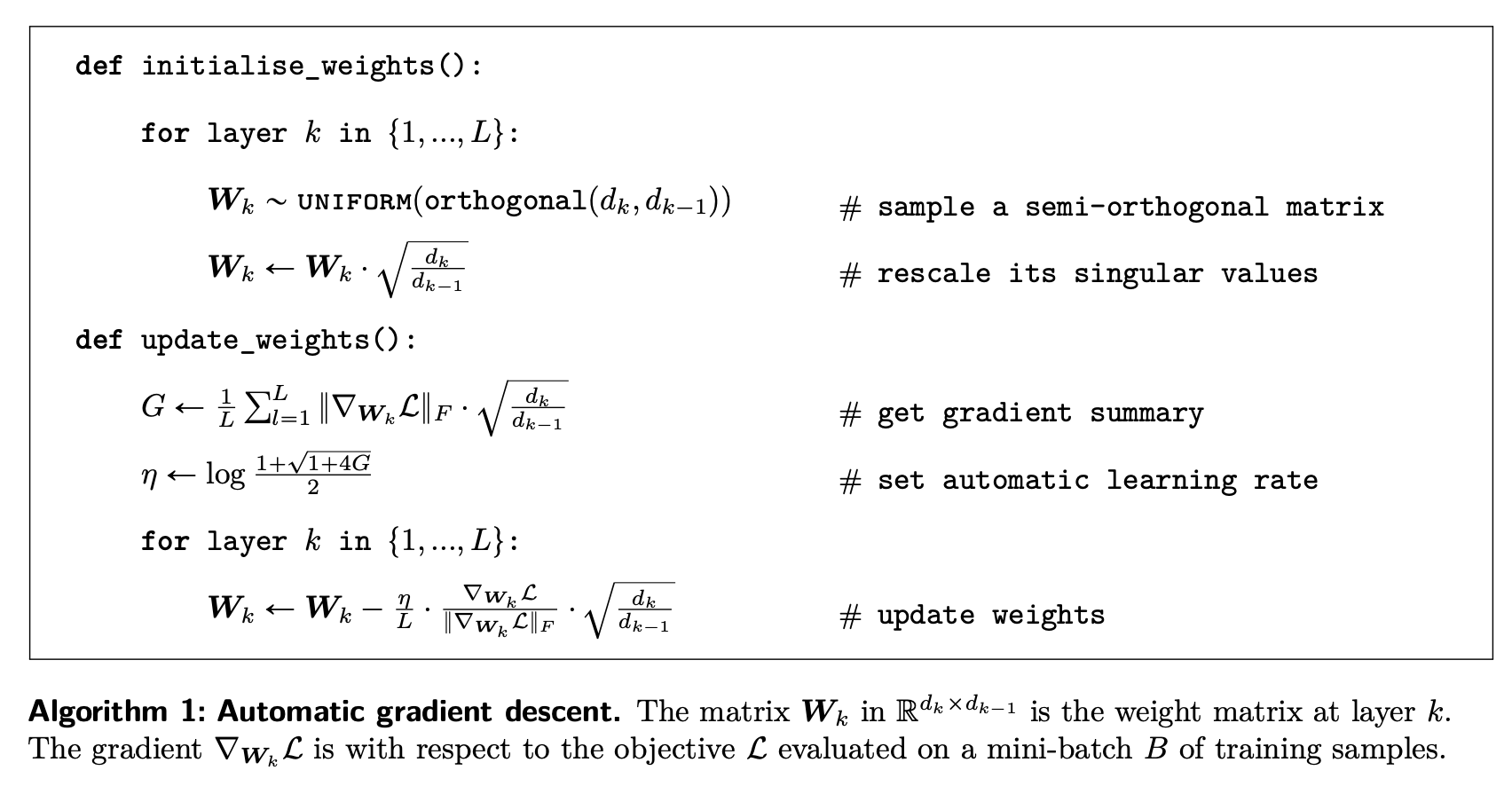
We include AGD in this discussion because it is an asymmetric algorithm: the weights are normalized in a layer-dependent fashion. In addition, it takes a stab at alleviating the annoying task of hyperparameter tuning. We see in practice, however, that it does not perform as well as Adam. This is presumably because the approximation of the loss function via upperbounding with matrix inequalities is not tight, or maybe because the model does not incorporate biases as presented in the paper.
We now begin discussion of our method, which has been crafted after studying these existing methods and taking into account the potential disbenefits of asymmetry.

Extension of AGD to regularized losses

We found the idea of AGD to be very nice, and in an attempt to understand it better, decided to explore one of the further directions listed in the paper: applying the method to regularized losses. The work in the paper applies to losses of the form $\frac{1}{N}\sum_{(x, y)}l(f_w(x), y)$. However, a more general loss includes a regularization term: $\mathcal{L}(w)=\frac{1}{N}\sum_{(x, y)}l(f_w(x), y)+\lambda R(w)$ where $R(w)$ is a regularization term. For our purposes, we assume $l$ to be the squared-loss and $R(w)$ to be the $L_2$ norm of $w$. We shorthand $\frac{1}{N}\sum_{(x, y)}l(f_w(x), y)$ to $\hat{l}$. Below, we derive the learning rate, in the context of AGD (i.e. with the spectrally normalized weights and same form of update), for this regularized loss:

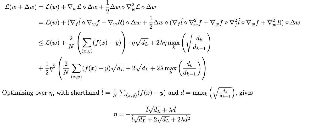
We have omitted a lot of intermediary steps involving matrix inequalities and derivatives - see the paper on AGD if you are interested in the details! We remark that this choise of $\eta$ depends on $\lambda$, so hyperparameter tuning is still necessary. Some dependence on the architecture shows up in $\eta$, namely $\Tilde{d}$. However, as the network scales this parameter can stay constant. We are interested in how this will perform in practice - check the blog for updates on this!

Introducing Asymmetric Nature

Our initial experiment involved a two-layer neural network (width: 1024) trained on the MNIST Dataset using three distinct learning algorithms: i) AGD (gain = 1), ii) Default Adam, and iii) Adam with diverse hyperparameters for both layers. The graph below showcases the resulting loss and accuracy. The first graph showcase loss while the second one showcase accuracy.

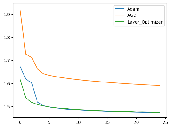
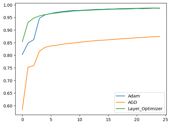
Given MNIST’s high accuracy even with minimal epochs, the distinction wasn’t apparent. Notably, while the asymmetric algorithm matched or outperformed default Adam, fine-tuning Adam’s hyperparameters yielded superior performance.

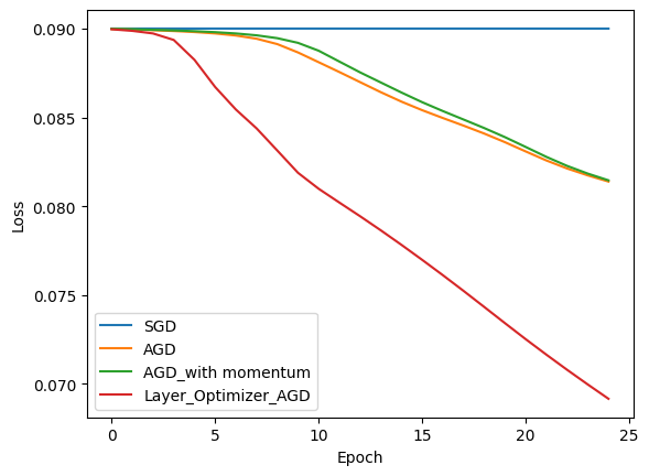
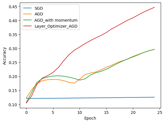
Inspired by AGD’s removal of the learning rate hyperparameter, we crafted two AGD variations for comparison with SGD and the original AGD.

Variation 1

This variation incorporated momentum into AGD, integrating AGD’s learning rate and gradient summary with momentum’s past and current gradients. Surprisingly, this had minimal impact, indicating the optimality of gradient summary and learning rate.

Variation 2

Here, instead of typical momentum, we introduced layer-wise asymmetry, acknowledging each layer’s varying impact on loss. Adjusting each layer’s learning rate inversely proportional to its number resulted in notable performance differences!

Results from training under these algorithms using the cifar-10 Dataset and MSE Loss are depicted in the subsequent diagram.

Evaluation Metrics

Emphasizing learnability, we adopt the ordering concept over exact measures. Algorithm $A_1$ is deemed superior to $A_2$ if its expected learning ability (distinguishing correct/incorrect classifications) surpasses $A_2$. This learning ability, resembling a Beta distribution, hinges on directly propotional to current accuracy. Therefore, we made our evaluation on accuracy and loss graph over epochs.

Conclusion

Our blog offers insights into optimizing neural networks and advocates for the potential benefits of asymmetry in training processes. We trust you found our journey as engaging as we did in developing it!

Citations

Ng, Andrew Y. ”Feature selection, L 1 vs. L 2 regularization, and rotational invariance.” Proceedings of the twenty-first international conference on Machine learning. 2004.

Bernstein, Jeremy, et al. ”Automatic Gradient Descent: Deep Learning without Hyperparameters.” arXiv preprint arXiv:2304.05187 (2023).

Kingma, Diederik P., and Jimmy Ba. ”Adam: A method for stochastic optimization.” arXiv preprint arXiv:1412.6980 (2014).

Philipp, George, Dawn Song, and Jaime G. Carbonell. ”The exploding gradient problem demystified- definition, prevalence, impact, origin, tradeoffs, and solutions.” arXiv preprint arXiv:1712.05577 (2017).