Structural vs Data Inductive Bias

Class project proposal

Introduction

Lack of Training Data

The transformative impact of vision transformer (ViT) architectures in the realm of deep learning has been profound, with their applications swiftly extending from computer vision tasks, competing with traditional neural network architectures like convolutional neural networks (CNNs). Despite their success, the intricacies of how architectural variations within ViTs influence their performance under different data conditions remain largely uncharted. Unraveling these subtleties

Project Goal

While much research has being made to find the best choice of data augmentation or the best structural change in the model to increase performance, our project empirically compares two kinds of methods:

• Data augmentation through tuning-free procedures
• Explicit inductive bias through discrete attention masking For data augmentation, we chose a simple-to-use procedure called TrivialAugment to increase by four times the amount of training data. Here we want an easy-to-use method that could help as a benchmark for the second method.

For explicit inductive bias, we use a general vision transformer architecture which allow us the change the number of attention heads and layers where the mask would be applied, this mask is what explicitly induce a bias in the model by forcing some layers to only learn relationship between close patches of the data.

Our goal with this comparison and the difference with previous works is that we want to experiment to which point one method could be better than the other by really compensating for the lack of information in the training of a vision transformer.

Due to computational and time limitations, we would train our model in a simple task of image classification based on CINIC-10. We also use a tiny model to be able to iterate many times through different scenarios of inductive bias. The selection of methods also reinforces these limitations but are a good starting point as many of the projects that would be lacking in training data probably are in testing phases where light tools like Google Colab are used.

Contribution

The result from this project contributes in two ways. First, it gives us a glance of how beneficial the level of proposed inductive bias in the performance of the model could be, and second, it contrasts which method, and until which point, performs better given different scenarios of initial training data available.

Related Work

Data Augmentation

Data augmentation consists in applying certain transformations to the data in order to create new examples with the same semantic meaning as the original data. For images, data augmentation consists in spatial transformations like cropping, zooming or flipping. Although data augmentation is very popular among practitioners, previous works like have proven that data augmentation by itself reaches a saturation point where it is even worse than training in the new data, decreasing the performance of the model. Given our goal of comparing data augmentation with inductive bias, we expect to get a similar result in the efficacy of data augmentation while we increase the initial amount of data.

Data augmentation decisions can be thought because of the many options available to perform, but it is so popular that some researches are trying to make it more easy to use and computational-efficient, one example been TrivialAugment method where simple random augmentation can be compared to or outperform other more complex algorithms that try to find the best augmentation for the given dataset. TrivialAugment would be the procedure used in this project given it simplicity.

Changes in Architecture

To compensate the lack of training data for vision transformers, an interesting approach from is to use instance discrimination techniques which adjust the loss function of the model to improve the representation of the datapoints getting high accuracy scores for datasets with only 2k samples. The model proposed is trained from scratch with few data, but its implementation and interpretability could be troublesome for small projects.

Othe authors in use a set of pre-trained models with complementary structures (Convolutional and Involutional) to help a lightweight visual transformer model called DeiT (Data-efficient image Transformer) increase its performance by getting a baseline result that is added as a token and works like an induced bias of the properties of the image. The scores from the pre-trained models give more information than the ground truth because it gives a value of likehood for every class, which is a result of the different attributes of the specific image.

Although these changes demonstrate that it is possible to get better performance with few data without augmentation, it is not clear how we can adjust the inductive bias produced to identify until which point it works. The usage of pre-trained models is also not desirable here because of our premise that we could be using this experiment to make decisions in new datasets and tasks.

Explicit Inductive Bias

The model proposed in is a better example of real lack of training data overcome by introducing a different kind of attention heads. In this case, medical images tend to have the same orientation, property that is leveraged to force the attention heads to focus on axial information which normally represents the spread of tumors. Here the inductive bias is that the image has a structure where patches aligned in rows and columns are more related between them than diagonal ones.

Following this path, , and try to apply the local induced bias of convolutional networks in a transformer by different methods. adds a new layer at the beginning of the model which acts like a local mask but with variable learnable attention levels, where the model figures out how much local attention it should apply given the proposed task. on the other hand add new convolutional layers in parallel to the transformer to let them capture the local information while letting the original transformer to keep the big picture of the image. Finally, in it is proposed a change in the initial attention layers, making them GPSA (Gated Positional Self-Attention) which learn for each patch if pay more attention to the attention product (Query * Key) or the position of the patch in the image.

From these works it is stated that some layers of the transformer converge to convolutional behaviors given the nature of the data used for training, but this requires a relatively big amount of data that could not be available. It is also noticed that the inductive bias is applied to the first layers of the model.

The model proposed in uses a simpler method which consists in applying a mask pattern to some of the attention heads to induce local attention bias into the model. To decide which heads and layers should be masked, it uses a soft masking approach where the model learns a scale factor between 0 and 1 which sets the level of local inductive bias that is applied to that head. The results show that it is possible to obtain good results by using more local masking in the first layers and keeping the global interaction in the last ones. This approach is also model agnostic and easy to implement, which is why it is close to the experimentation of this project.

The power of this masking method is also shown in where the mask is learned by a parallel process of pixel-wise classification, successfully increasing the performance in more complex tasks like pixel-wise segmentation.

Methods and Experiment

To explore and compare the benefits of data augmentation versus induced bias we are running three related experiments. All experiments would be run with CINIC-10 dataset in Google Colab using a T4 GPU. We decided to use CINIC-10 instead of CIFAR-10 because even though it is a drop-in replacement of CIFAR-10, it is a much larger than CIFAR-10 so we can test on different number of base training samples but not so large like ImageNet that is too large/difficult to test.

Experiment 1

The goal of the first experiment is to get a glance of the overall differences in accuracy for the compared methods. The model used for this experiment consists of a basic visual transformer with six layers and linear positional embeddings. Each layer corresponds to a multiheaded attention layer with only two heads. The schematic of the model can be seen in figure 1.

Figure 1

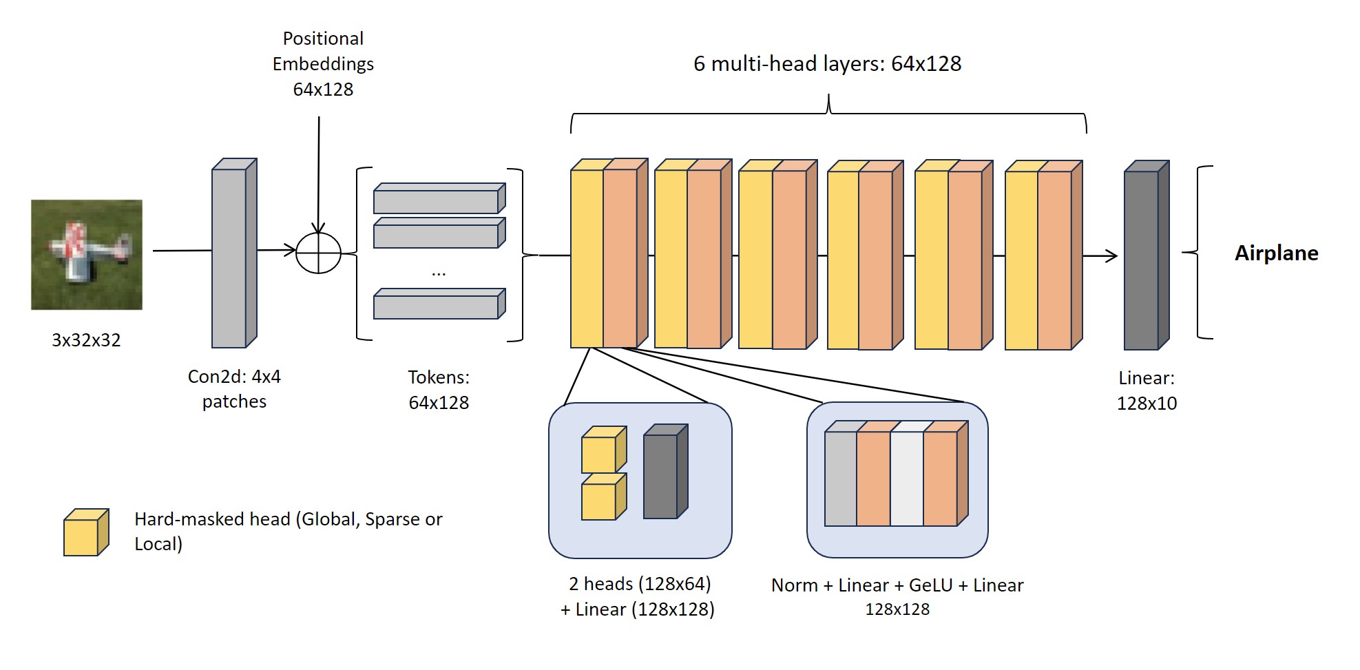
By default, the attention heads in the model are fully connected to give them a global behavior, but the model can be configured to apply a local pattern mask or a sparse pattern mask to all heads in all layers.

Figure 2

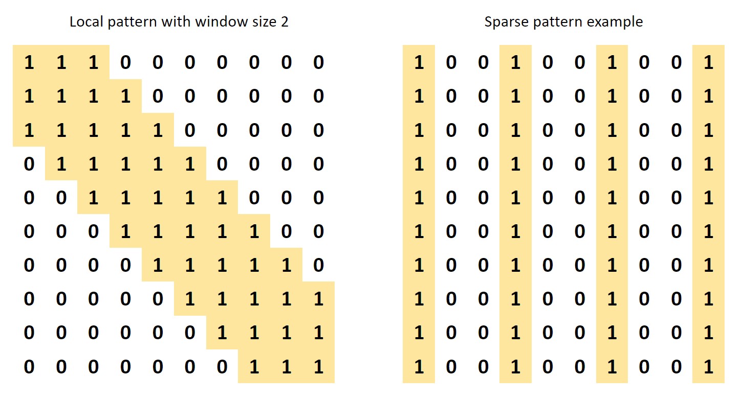
The model would be trained with different scenarios of initial data, in specific, with 1000, 2000, 5000, 12500 and 20000 samples. In each scenario, we would get four different models:

• Baseline model: Without data augmentation and with default global attention
• Data augmentation: With data augmentation and default global attention
• Local attention: Without data augmentation and with local attention
• Sparse attention: Without data augmentation and with sparse attention

The data augmentation technique would be TrivialAugment and the metric would be accuracy on validation dataset. We set these four models trying not to mix data augmentation with changes in the induced bias, keeping the default global attention in the transformer as our baseline.

Experiment 2

Having experimented with the differences where all layers have the same mask, we now set experiments to play with the level of induced bias applied to the model. The goal now is to identify a relation between the level of induced bias applied to the model and their performance. For this experiment we modify our first model in the following ways:

• We increase the number of attention heads in each layer from 2 to 4
• We set the final two layers to global attention, so the mask is not applied to them
• We configure each head in the first four layers to be able to be hard configured as either local or global attention.

Figure 3

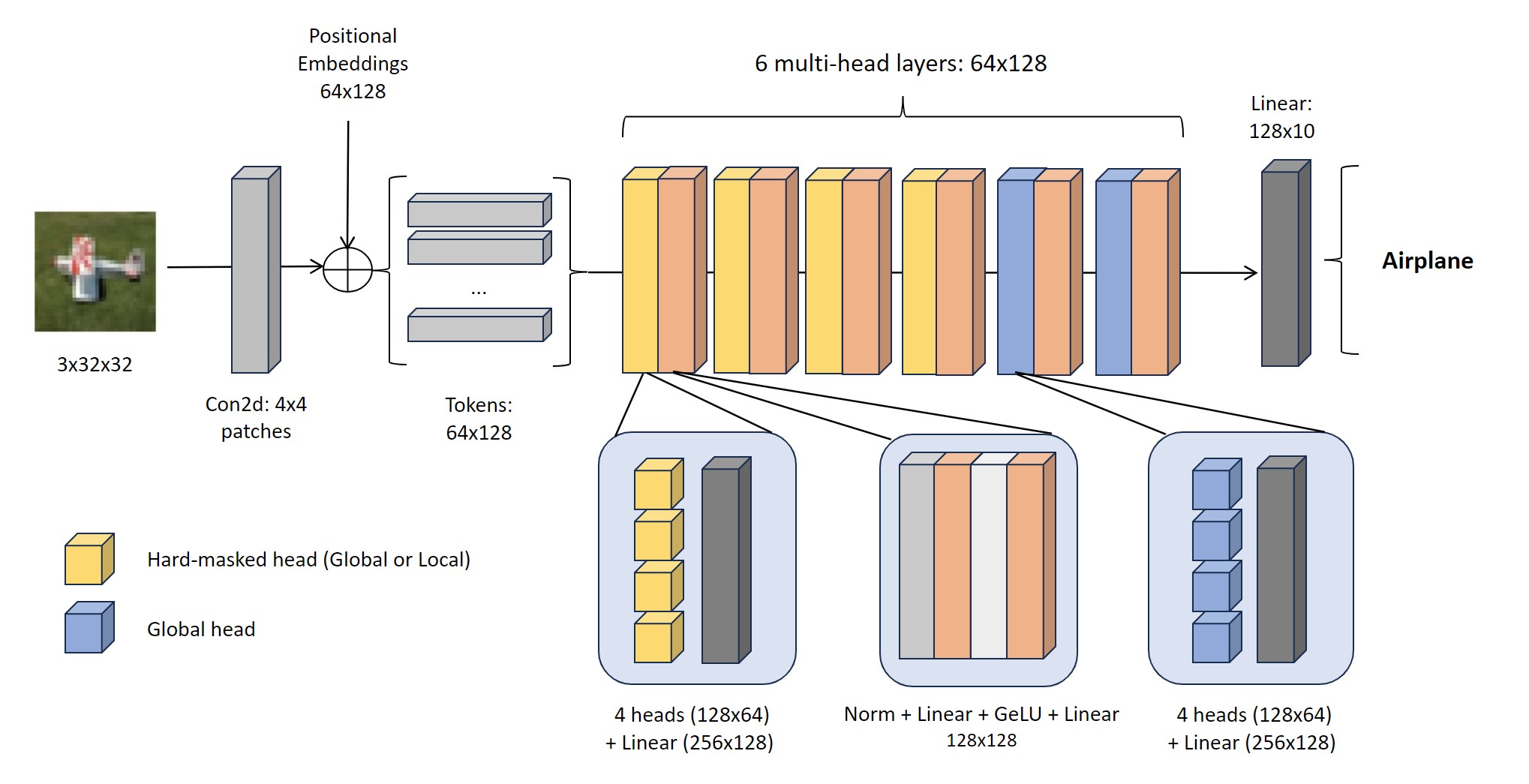
With this new model, we can create one instance for each combination of global/local head in any of the first four layers, generating a sense of “level of induced bias” based on the number and configuration of attention heads treated as local.

Given computational limitations, we would set only two initial data scenarios (10000 and 50000) and get 16 models for each scenario:

• Baseline model: Without augmentation and with all global attention
• Data augmentation: With data augmentation and all global attention
• 14 combinations of local heads and layers:

Table 1

We would analyze the differences in accuracy between different levels of induced bias in the same initial data scenario and see if we can get a selection of best performing inductive bias levels to apply them more broadly in the third experiment.

With this comparison we also want to capture what are the visual differences between the attention heads in the different levels of induced bias to try to explain with is doing better or worse than the baseline.

Experiment 3

Our final experiment consists in comparing the accuracy and the effective additional data (EAD) that each method brings when applied to different initial amounts of data. The initial data scenarios to train the models would be 1000, 5000, 10000, 20000, and 50000 samples. The comparison would be made between the data augmentation model for each scenario, versus the top 3 levels of induced bias from experiment 2.

The effective additional data (EAD) represents the extra amount of real data that the method is compensating, the higher the better to be considered as a successful method for solving lack of data problems. This metric is calculated by looking at which scenario of initial data would make the baseline model perform equal to the method analyzed.

Results

Experiment 1

In our initial experiment, we compared performance on four variations of model scenarios. Our baseline model uses global attention mechanism, one uses local attention mechanism, another one uses sparse attention mechanism, and the last model uses the same global attention mechanism as the first model except that data augmentation is applied during its training process. One notable callout for our initial experiment is that we took a naïve approach and designed our local and sparse attention heads to be in all six attention layers of the attention. We trained and collected the validation accuracy and training time for each model variation for different number of base training samples from 1000 to 20000. Below are the results.

Result and Analysis

Figure 4

Figure 5

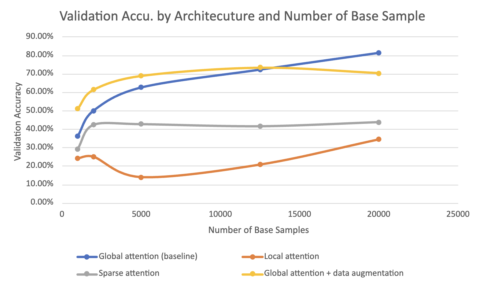
There are a few notable observations to point out from the results. First, we can see that the two models using the local attention mechanism or sparse attention mechanism performed significantly worse than our baseline model that used global attention. Though we did expect this to happen since CINIC-10’s classification task intuitively requires a global context of the image, we did not foresee the performance difference to be so drastic. For example, when the base number of training data is 5000, we see that the baseline model achieves a validation accuracy of 62.5% while the local attention model achieves just 13.97% and the sparse attention model 42.64%. We observe a similar pattern across different levels of base samples. It’s also worth calling out that sparse attention models perform better than local attention models. This makes sense as sparse attention models still take into consideration the global context just not completely on all the patches. Nevertheless, the sparse attention model takes almost the amount of time to train as the baseline model, hence it does not make sense to use it in lieu of the baseline model in practice. On the flip side, we verify that data augmentation improves performance and is the most significant when number of base samples is small.

Experiment 2

Our first experiment showed that simply setting all attention layers to contain only local or sparse attention heads does not produce good performance. As we were exploring additional datasets or tasks where applying a different attention mechanism may yield better performance, we came across the paper in , in which it alluded to the idea that only applying local attention mechanism to just a few beginning layers of the network may improve performance even when the task intuitively requires a global context. The rationale behind it is that perhaps through using local attention mechanism, the model can create its own convolution making understanding local information better before using that information to answer a task that requires global context. With this inspiration, we designed our second experiment trying out different combinations of local attention heads and layers, as described in the Methods and Experiments section, and below are the results and analysis.

Result and Analysis

Figure 6

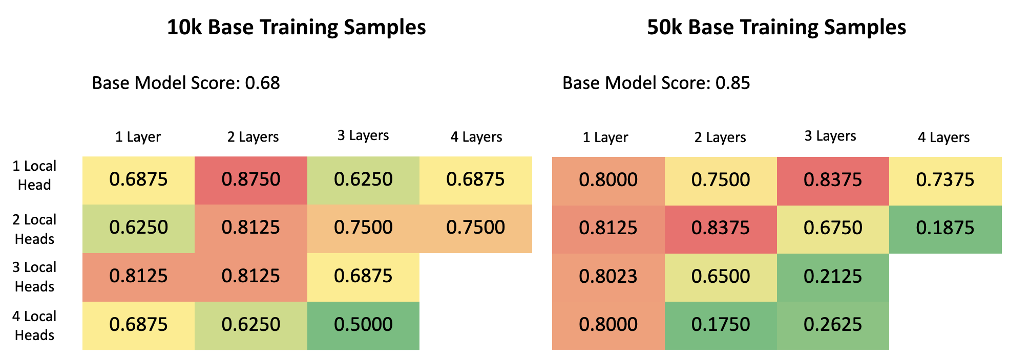
Here, the two matrices outline the validation accuracies we got when we trained the different local attention mechanism model on 10k and 50k base training samples. A quick recap, 1 Local Head and 1 Layer means we would use 1 local attention head in the 1st layer of the transformer. The color gradient in each matrix indicates the best performing combination from best (red) to worst (green).

A few patterns can be noticed. First, for both matrices, models in the bottom right corner, representing a high number of local heads and in more layers, are performing worse than the rest. This aligns with our intuition from our first experiment because having more local attention heads in deeper portions of network will prevent the models from capturing global context, thus resulting in a worse performance.

Figure 7

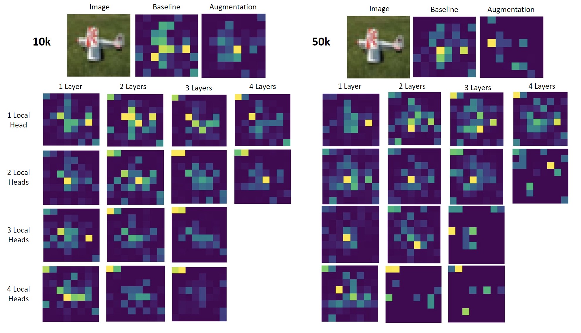
Diving further, in figure 7, we visualize the attention weights to better compare different levels of induced bias. It seems that the performance increases as we add more local heads, but it ends up fading and not capturing the important characteristics of the data. In the 50k samples scenario it can be noticed that with more local heads, the attention spots converge to small parts of the image where there is no information about the object in it.

Figure 8

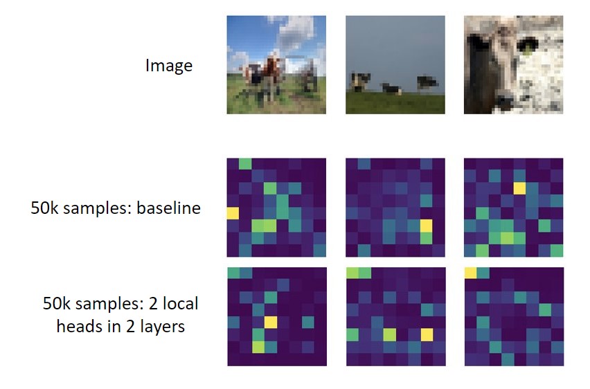
Moreso, in figure 8, it can be noticed that when local heads are used, it identifies correctly smaller details of the image. In this case, with all heads being global, it is hard to identify the three different cows in the middle image, but when some local heads are used, we can capture them.

In summary, the major result of this experiment is that some models in the 10k samples sub-experiment produced better results than the base model. This is promising and validates our hypothesis from before. Though no combination produced better results in the 50k samples sub-experiment, we showed in Figure 8 that having local attentions can still be beneficial as it is able to capture some details that the baseline model misses.

Experiment 3

From the second experiment, we were then intrigued to see how some of the better performing models do under different number of base samples than just 10k and 50k. So, we pick three combinations (2 local heads for 2 layers, 1 local head for 2 layers, 3 local heads for 1 layer) and tested their performance against the baseline model and baseline + data augmentation for different number of base training samples from 5000 to 50k. Below are the results and analysis.

Result and Analysis

Figure 9

Figure 10

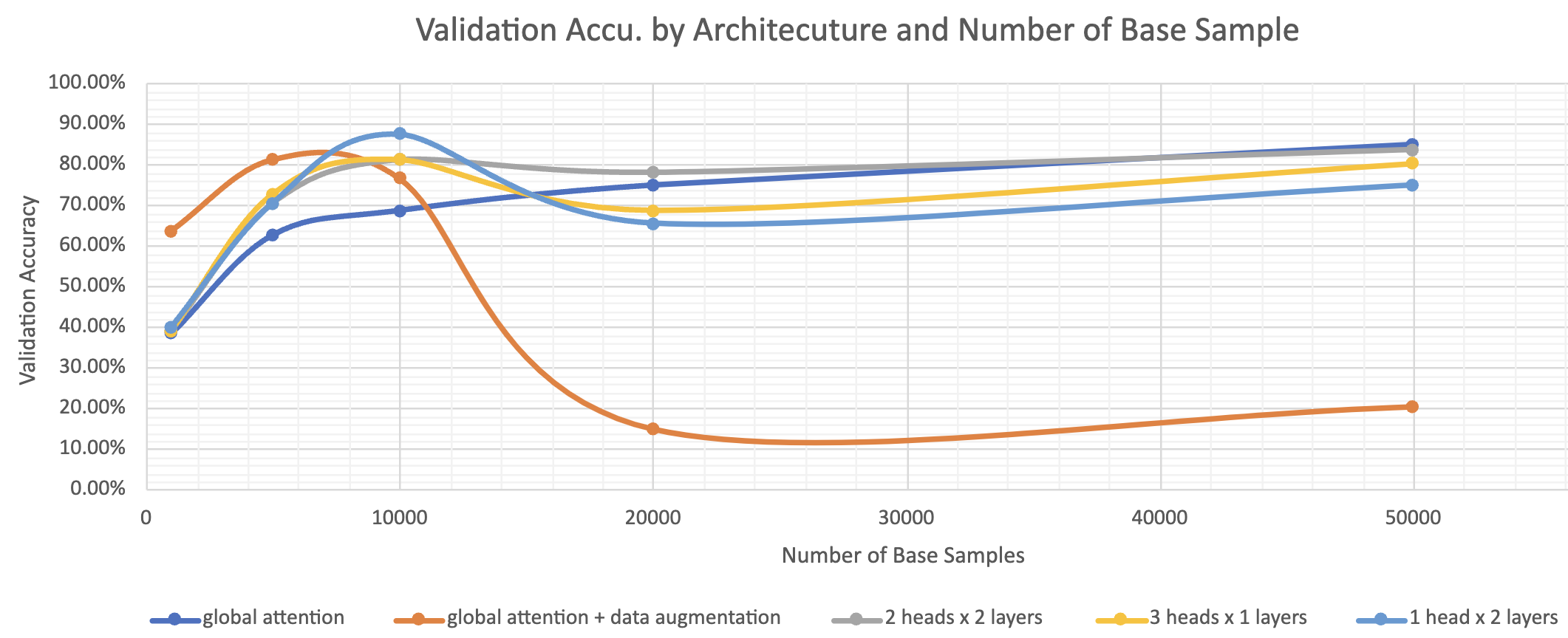
Here, we can observe two very interesting trends. First it validates our hypothesis that using local attention heads early in the layers of the vision transformers can improve performance despite the fact that task intuitive requires global context. This outcome is true for all three variations of the local attention models when the number of base training samples are 1000, 5000, and 10000. However, this effect tapers off when the number of base samples is sufficiently large, and the baseline model performs better. This seems to suggest that the benefit of the inductive bias coming from the local heads no longer outweighs the lack of information of the dataset. In other words, once there is sufficient data, the baseline model has enough information to learn a better representation on its own than that of the models.

Figure 11

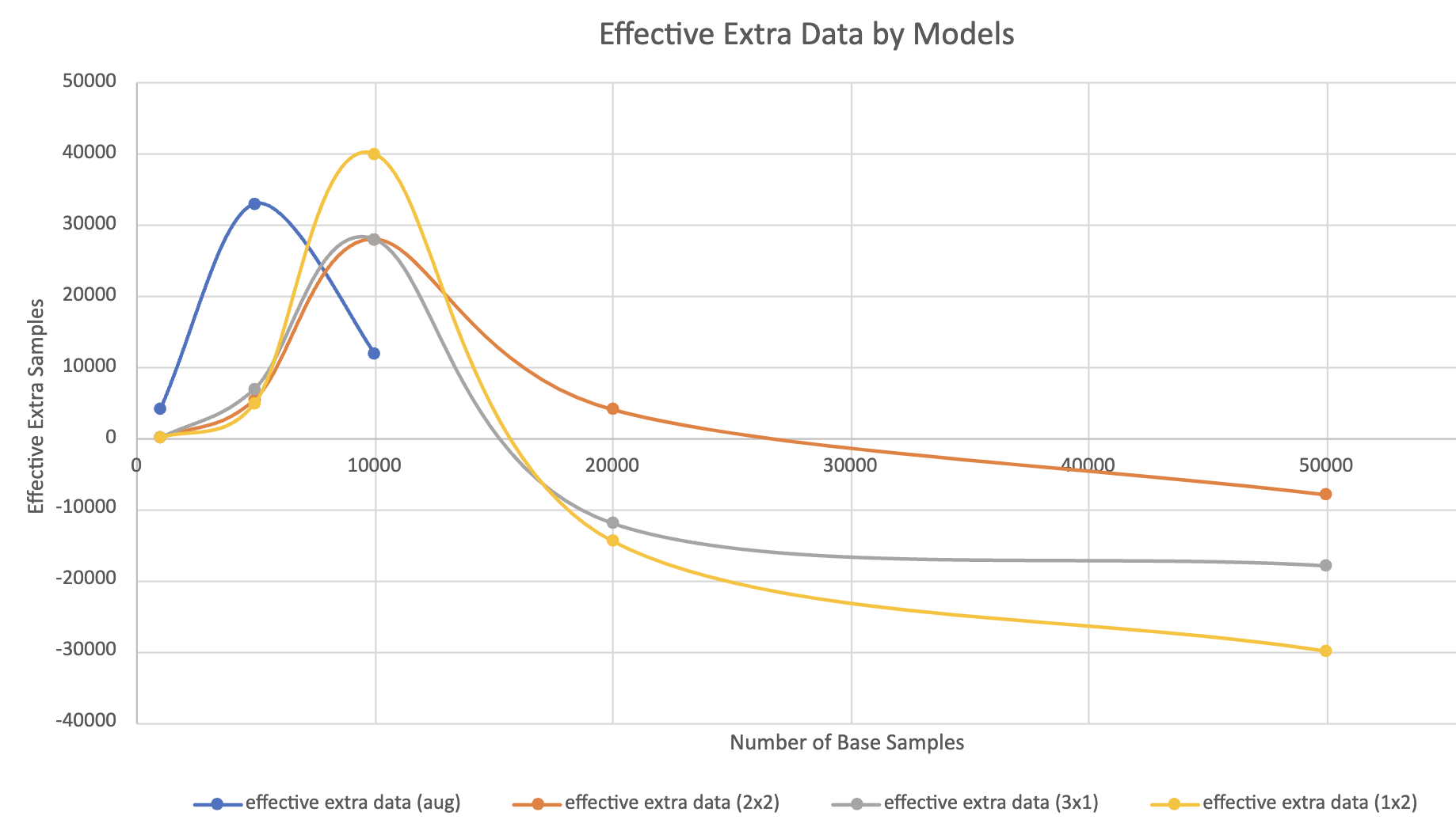
Another perhaps more explicit and comparable way of explaining the phenomenon is to look at the Effective Extra Sample score. Essentially, the data tells us how much extra (or less) training data the change in model architecture gets us to achieve the same performance accuracy if using the baseline model. This graph clearly illustrates that data augmentation and tuning of local attention heads are very effective when the training datasets are relatively small, less than 15000 samples. This is likely because the inductive bias of the local attention heads causes the models to capture important characteristics of the image more efficiently and effectively than does the baseline model. However, once the number of base training samples gets over 20000, the effect reverses and they all perform worse than the baseline model, as illustrated by the negative effective training samples.

Note: We did not plot the extra effective data for the data augmentation model scenario pass 10000 base training samples as its performance dropped significantly and is behaving weirdly.

Conclusion

Through different experimentations, both data augmentation and induced bias by discrete attention masking can compensate for the lack of data for a given problem, but this compensation is only noticeable when the initial data is very low.

The maximum effective additional data that the data augmentation method creates is higher than the induced bias method, but there is a sweet spot where induced bias is better than both data augmentation and baseline model.

Once the initial amount of data starts to increase, data augmentation is the first one that in fact worsens the performance of the model. Induced bias on the other hand looks more stable while the initial data is increasing but is still not significantly better than the baseline model.

We have shown that induced bias can help identify local attributes of the image more easily than the baseline alone, but this is only leveraged when the task that we want to solve is more specific and cannot be appreciated in a general task like image classification.

Limitations and Next Steps

Given the restricted resources and amount of time available to execute this project, there is enough room for continuing research on this topic:

• We tried to make the data augmentation and inductive bias methods simple and easy to play with, but they could not be the best ones. The same procedures of this project can be applied to better and more complex types of data augmentation and induced bias to see if the results are replicable in other situations.
• Further experimentation could be done with datasets with multiple tasks and a deeper model to see if the type of task has an impact of the effectiveness of one method or the other. This could also be applied in recent real-world problems where there is not enough data yet, but we can clearly identify the relying relationship between patches of the images.
• Given a deeper model and a lot more experimentation in the level of inductive bias, there is an opportunity to empirically try to make a regression between how much inductive bias is applied to the model vs the resulting change in performance. The results of this project are not enough to implement such relations.