Robustness of self-supervised ViT features in b-mode images

Vision Transformers (ViT) trained with self-distillation with no labels (DINO) have shown striking properties for several downstream tasks regarding segmentation, classification, and image correspondence. In this work, we assess DINO-vit-s/8 on a new dataset containing b-mode ultrasound images with the ultimate goal of segmenting bone.

Introduction

B-mode ultrasound imaging is a widely employed medical imaging technique that uses high-frequency sound waves to produce visual representations of the internal structures of the human body. Its main advantages are its ability to produce real-time images, its portability, low cost, and especially the fact that is noninvasive and safe (non-radiating). However, it is an imaging modality that carries a very high noise-to-signal ratio. Speckle noise, out-of-plane movement, and high variability in image reconstruction across devices make the resulting images complex to interpret and diagnose . As an example, the following figure shows an annotated b-mode ultrasound image.

Ultrasound b-mode image of the upper arm with the main physiology annotated.

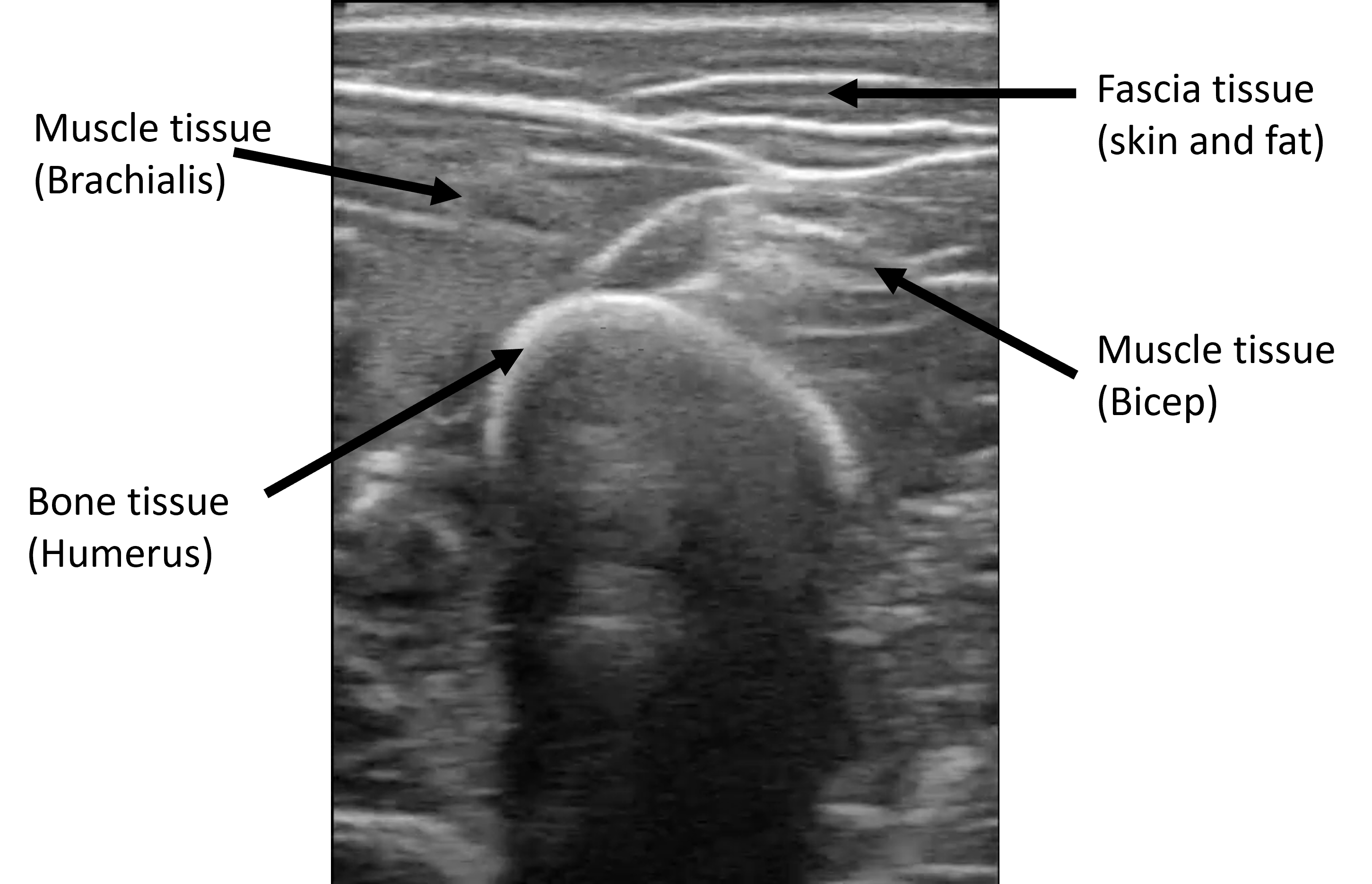
Self-supervised Vision Transformers (ViT) have emerged as a powerful tool to extract deep features for a variety of downstream tasks, such as classification, segmentation, or image correspondence. Especially, DINO architectures have exhibited striking properties, where its deep features present localized semantic information shared across related object categories, even in zero-shot methodologies . Consequently, the aforementioned properties of DINO may allow us to develop efficient yet simple methods for b-mode ultrasound image interpretation, without the need for an expert or ground truth labels.

In this work, we propose analyzing the performance and robustness of DINO in b-mode ultrasound images of the arm and leg, capturing musculoskeletal tissue from two different ultrasound devices. We note that this dataset features a series of images with a high noise-to-signal ratio, which is a property that DINO has not yet been tested against. In particular, we focus on assessing DINO-vit-s/8 deep features across its blocks as well as its attention weights, with the final objective of segmenting bone on b-mode images in a zero-shot approach. Through all these experiments, we show the potential and feasibility of implementing DINO models in real-world b-mode medical imaging applications.

Related Work

DINO-vit Assessment

Since the release of DINO, a self-supervised method for training ViTs based on self-distillation, there has been a line of work focused on exploring new capabilities and assessing the deep features obtained from such pre-trained models. In , they showed how the attention heads corresponded to different parts of an object in an image, or how one could segment desired objects by thresholding the self-attention maps. Similarly, semantic information analysis across related images was performed to show the potential of the deep features contained in DINO-vit models. Employing principal component analysis (PCA), matching algorithms or linear classifiers on the deep features, promising results on segmentation, semantic co-segmentation, and correspondence tasks were presented , .

Further research was done by combining Stable Diffusion features and DINO features, improving semantic correspondence tasks at the cost of increasing the computation effort . While DINO has shown strong generalization to downstream tasks, there has been no work on the assessment of this model on a b-mode ultrasound imaging domain. Besides the high signal-to-noise ratio, ultrasound images usually present a complex structure of tissues that makes it difficult to differentiate between the foreground, the desired structure to segment or analyze, and the background. Our work shows that DINO is also robust to this type of images, leading to promising results on segmentation tasks.

Ultrasound B-mode Imaging Segmentation on Musculoskeletal Tissue

Muscle and bone segmentation have important applications in clinical and rehabilitation practices to assess motion performance, diagnosis of the musculoskeletal system, and quantification of rehabilitation procedures, among others. There has been effort in developing deep learning tools to automatically segment and quantify desired parameters for the aforementioned applications. In , a U-Net architecture with Deep Residual Shrinkage layers for denoising was implemented and trained to segment muscle fibers. Similarly, different muscle heads were segmented employing a large dataset of muscle images from different subjects and devices to train several convolutional neural network architectures , .

Medical images, from any source, are in general scarce and difficult to label, which poses a limitation for deep learning models to achieve a good performance and generalization. Most of the current methods, lack the capability to perform well in unseen segmentation tasks involving different anatomies. In , they developed a deep learning model, UniverSeg, based on a novel Cross-Block mechanism that produces accurate segmentation maps without the need for additional training. However, when employed in noisier data domains, such as b-mode images, the performance breaks down. In this work, we discover that DINO has potential even when dealing with noisier datasets based on b-mode ultrasound images.

Methods

Dataset

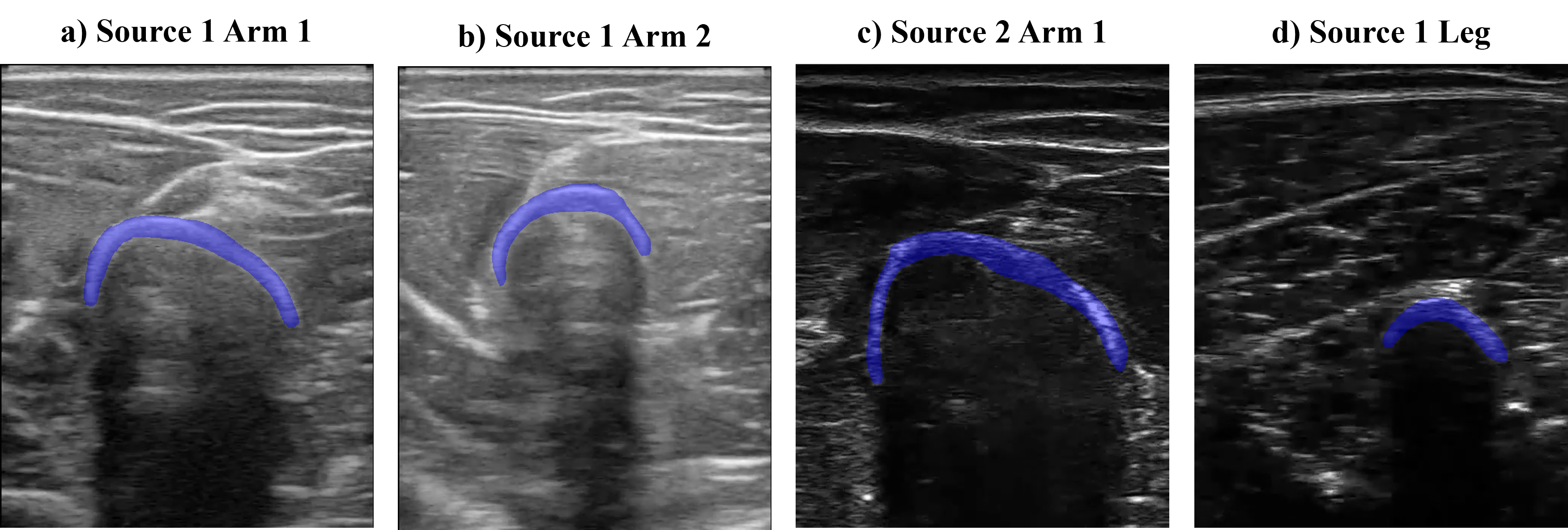
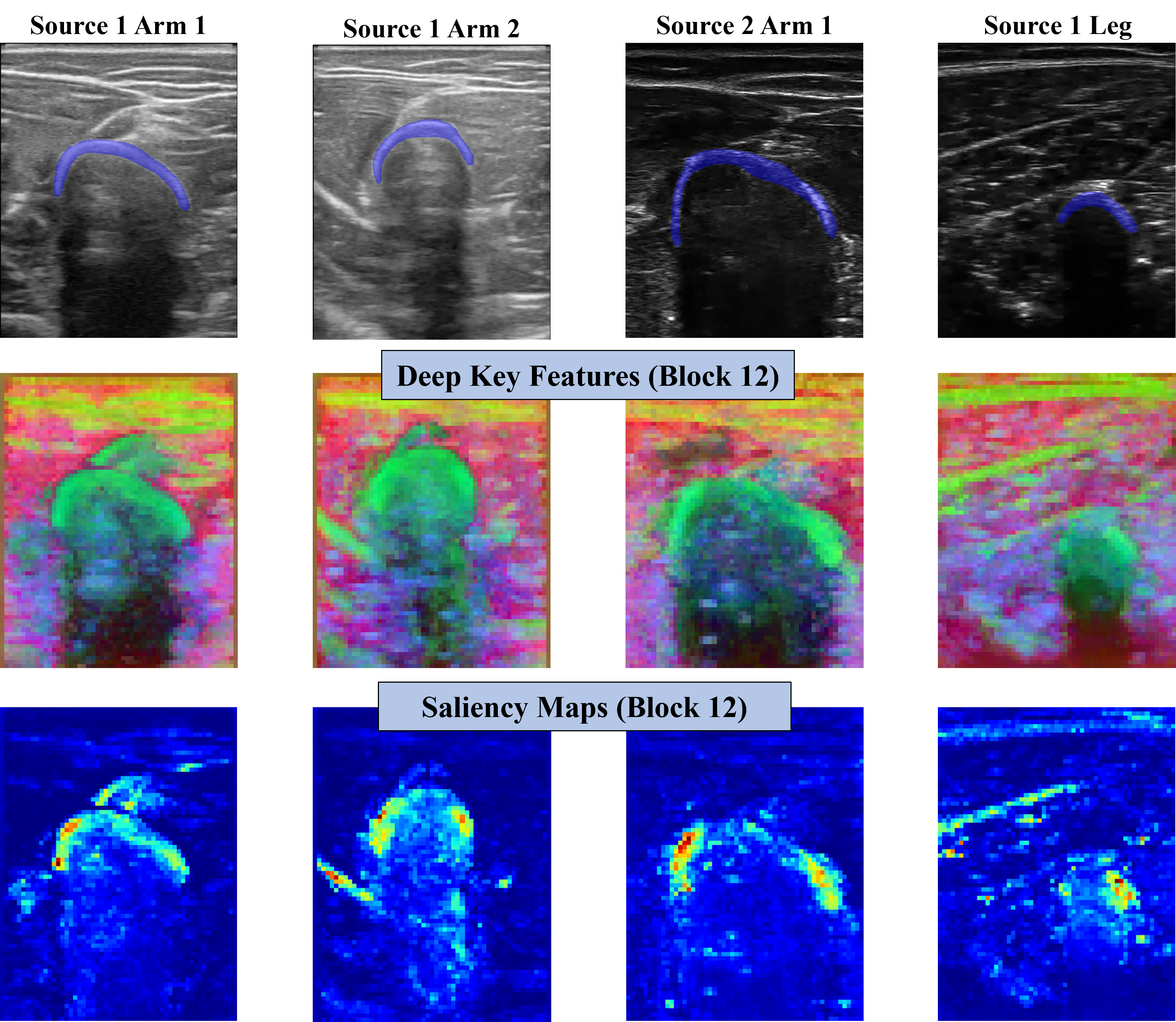
The dataset consists of b-mode ultrasound images from the arm and leg of two subjects while moving. We recorded short videos and randomly selected frames to obtain the images. In the images, bone, muscle, and fascia tissues can be appreciated. We also acquired videos from two different ultrasound sources to expand the domain where DINO was tested. With all this, 4 different image origins (or image domains) form the dataset, as appreciated in the figure below. We labeled 10 bone heads of each domain to evaluate DINO’s performance.

Example of one image of each origin with its mask label (blue). a) Arm (Source 1, Subject 1). b) Arm (Source 1, Subject 2). c) Arm (Source 2, Subject 1). d) Leg (Source 2, Subject 1)

Deep Feature Assessment

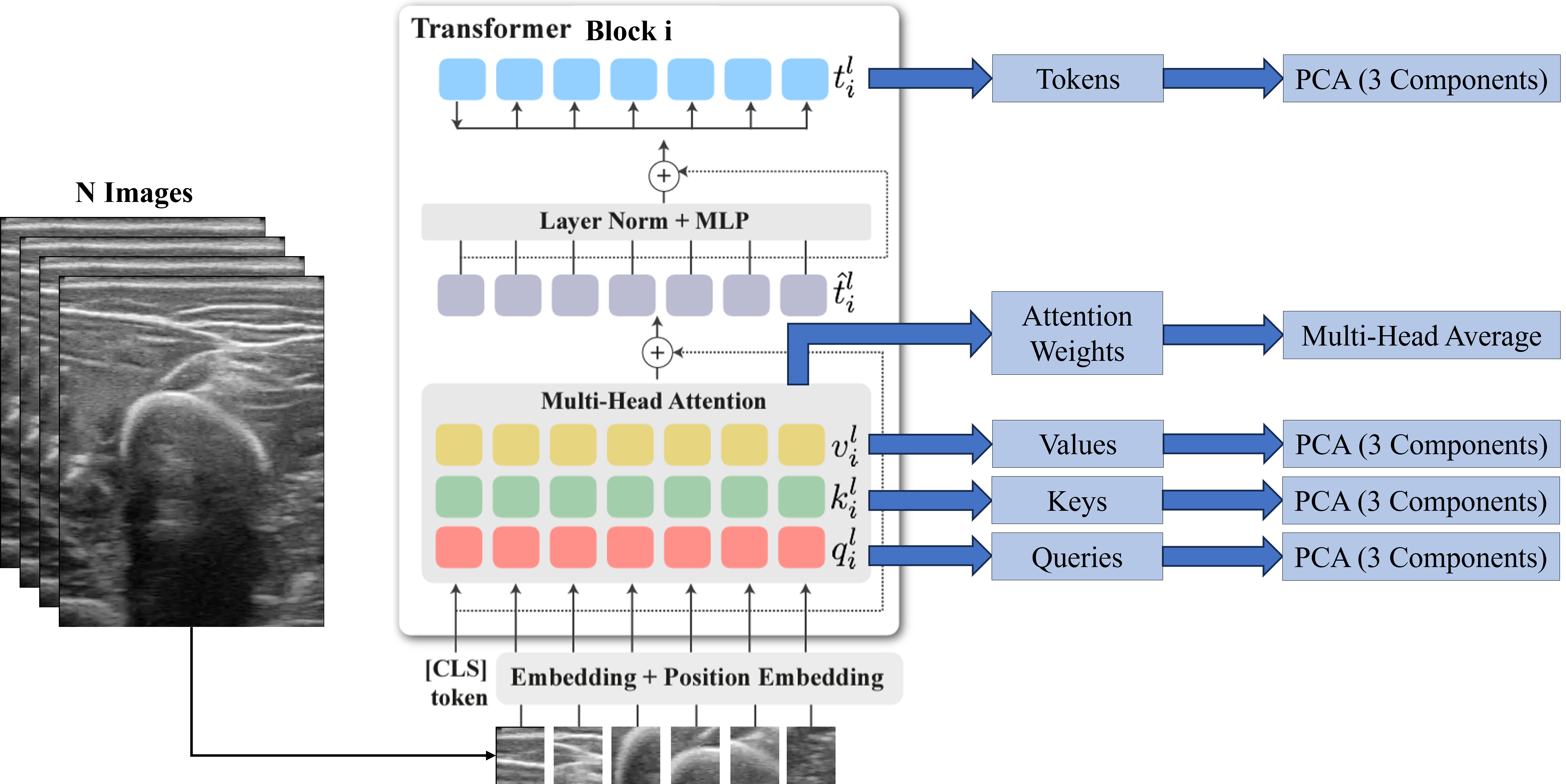
We analyzed DINO-vit-s/8 features over different layers qualitatively. For any block \(i\), we extracted the Keys, Values, Queries, and Tokens and applied a principal component analysis (PCA) to get the three most important components. For the attention maps, we averaged the self-attention weights of the CLS token over each head of the multi-head block.

This analysis was done with the intention of qualitatively finding the most suitable deep features for the subsequent segmentation task. Similarly, the self-attention maps were observed to corroborate that the model focuses especially on the bone, and less on the surrounding structures.

Workflow to obtain deep features as well as self-attention information. Transformer block design obtained from .

Segmentation Pipeline

As described in the results section, the Keys of the last block (block 12) of DINO-vit-s/8 were employed as deep features for the segmentation. As in , we used a zero-shot approach as the pipeline for bone segmentation. We first clustered together all the features obtained from the different images passed through DINO with k-means. Then, we selected those clusters for the segmentation mask employing a simple voting algorithm. Being \(\texttt{Attn}_i^\mathcal{I}\) the self-attention of the CLS token averaged over all heads of block 12 in image \(\mathcal{I}\) and patch \(i\); and \(S_k^\mathcal{I}\) the segment in image \(\mathcal{I}\) belonging to cluster \(k\). The saliency of this segment was computed as

\[\texttt{Sal}(S_k^\mathcal{I}) = \frac{1}{|S_k^\mathcal{I}|} \sum_{i \in S_k^\mathcal{I}} \texttt{Attn}_i^\mathcal{I}\]

and the voting of the cluster \(k\) was obtained as

\[\texttt{Votes}(k) = \mathbb{1}[\sum_\mathcal{I}\texttt{Sal}(S_k^\mathcal{I}) \geq \tau ]\]

for a threshold \(\tau\) set to 0.2. Then, a cluster \(k\) was considered to be part of the mask if its \(\texttt{Votes}(k)\) were above a percentage of 65% of all images. The following image sketches the whole process.

Zero-shot segmentation pipeline using keys as deep features.

To quantitatively assess the segmentation results, both Dice and IoU metrics were computed employing the labeled bone head segmentations.

Results

Deep Features Assessment

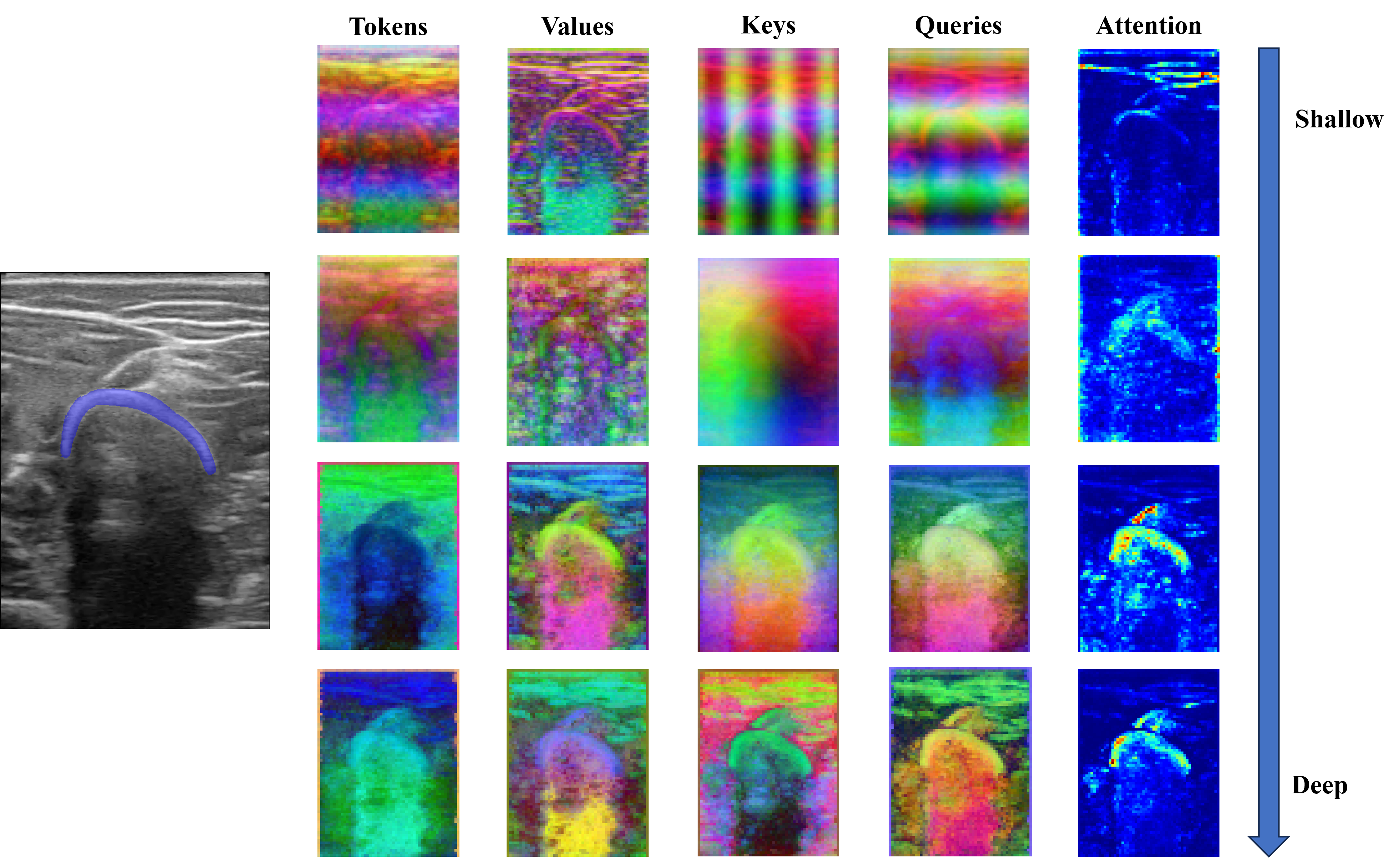
We first input a single image to the model and analyzed the Keys, Values, Queries, and Tokens, as well as the self-attention of the CLS token from shallower to deeper layers.

The three most important components after performing the PCA on the deep features are plotted in RGB as depicted in the figure below. Tokens seem to carry spatial information throughout the different blocks, representing depth information in the final block. On the other hand, Keys and Values seem to carry spatial information on the shallower blocks, and semantic information on the deeper blocks. In fact, we considered the Keys descriptors the most appropriate to be used to segment bone, as the bone head can be distinguished from the surrounding structures. Regarding the attention maps, they seem to move from the skin (in shallow blocks) to the bone (deeper blocks).

Token, Value, Key, and Query features as well as self-attention maps for different blocks (from shallow to deep).

Now, if we focus on the Keys features of the last block for the four different image domains, we can appreciate a similar behavior. Bone heads seem to be represented in all four cases by the Keys, being differentiated by the surrounding structures. That being said, we should note that the intersection between muscles just above the bone is in some cases also represented like the bone. Regarding the self-attention maps, in all four cases, they are principally focused on the bone head. However, we can also see that some muscle fibers or intersections may be present.

Keys deep features and self-attention maps from block 12 for the four different image origins.

An interactive scatter plot is another method to argue the representation of the bone by the Key features. For all the four different image origins, the patches belonging to the bone head are grouped on a region of the Euclidean space, while the patches belonging to other structures are scattered all over other regions.

3D scatter plot of the 3 components of the Key descriptors (block 12). Legend: "other" any patch not belonging to the bone head. "boneS1A1" bone patches of Source 1 - Arm Subject 1. "boneS1A2" bone patches of Source 1 - Arm Subject 2. "boneS2A1" bone patches of Source 2 - Arm Subject 1. "boneS2L" bone patches of Source 2 - Leg Subject 1.

Same Domain Experiment

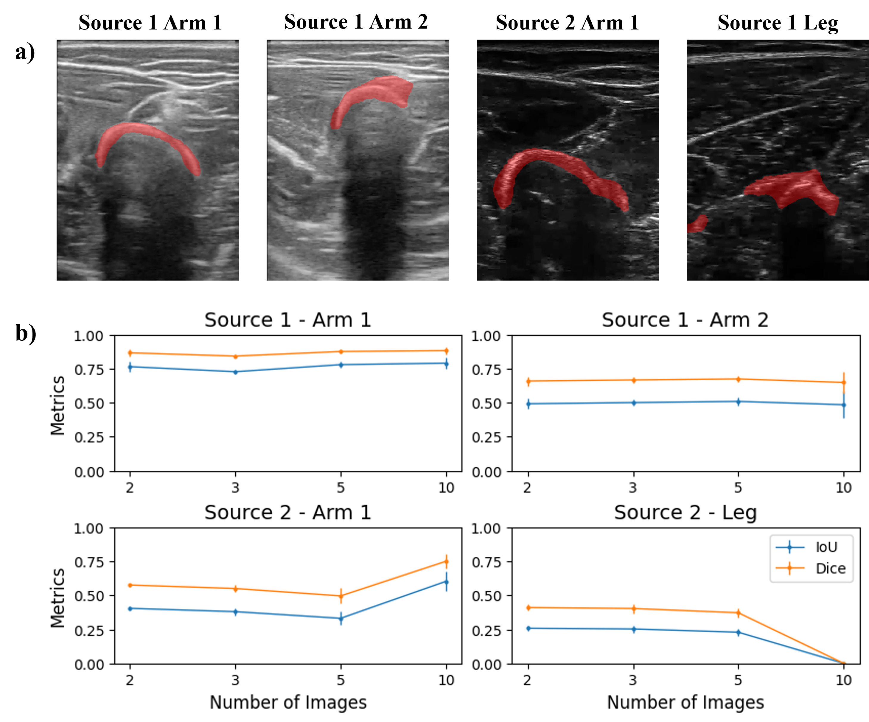
We subsequently performed the segmentation task on a set of images from the same origin. For each of the 4 domains, sets of 2, 3, 5, and 10 images were input to the segmentation pipeline. Recalling that the images were selected as random frames from short videos, each image within a domain presented a slightly different configuration of bone and surrounding structures. Therefore, the goal of segmenting with varying image quantities was to evaluate the balance between improvements due to increased feature quantity versus confusion introduced by variation in the images.

The reader can observe the results in the figure below. The bones from Source 1 Arm 1 are the best segmented, and the amount of images does not affect the performance, obtaining constant values of Dice and IoU of about 0.9 and 0.77, respectively. The segmentation of images from Source 1 Arm 2 in general takes also some part of the muscle tissue, and as in the previous case, the amount of images used does not change the performance with Dice and IoU metrics of about 0.7 and 0.5, respectively. In the case of images from Source 2 Arm 1, a larger quantity of images improves the segmentation results, increasing Dice and IoU metrics from 0.58 to 0.75, and 0.46 to 0.61, respectively. Finally, the segmentation masks from images from Source 2 Leg carry not only the bone but part of the surrounding tissue too. When increasing the number of images to 10, the performance drastically falls (with Dice and IoU of 0) as the segmentation results contain muscle fibers instead of bone.

Results of the segmentation on same domain images experiment. a) Segmentation result examples for the 4 different image domains. b) Metrics for the 4 different image domains and different amounts of images (mean and standard deviation).

Different Domain Experiments

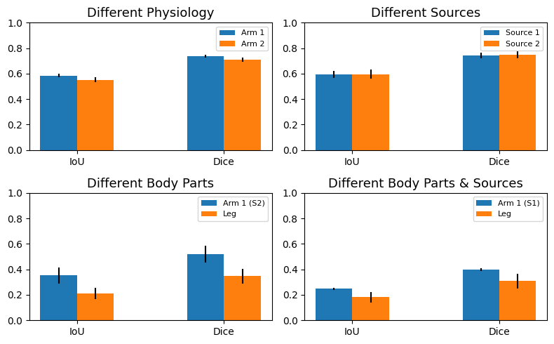
Then, we performed the segmentation task on a set of images from origin pairs. Five images of each origin were paired forming the following groups. Group 1: different physiology (source 1 - arm subject 1 and source 1 - arm subject 2), group 2: different sources (source 1 - arm subject 1 and source 2 - arm subject 1), group 3: different body parts (source 2 - arm subject 1 and source 2 - leg subject 1), and finally group 4: different body parts and sources (source 1 - arm subject 1 and source 2 - leg subject 1). We carried out this experiment to evaluate if the deep features shared from different image origins were similar enough to properly perform the segmentation task, giving an idea of feature correspondence between different image domains.

The image below shows the experiment results. The segmentation performed on the domain source 1 arm subject 1 worsens when paired with any other image domains. Both IoU and Dice metrics fall from 0.9 and 0.77 (previous values) to 0.78 and 0.59, respectively. Contrarily, the domains consisting of source 1 arm subject 2 and source 2 arm subject 1 improve when paired with source 1 arm subject 1. Finally, the image origin containing leg images maintains a similar segmentation performance when being paired.

Results of the segmentation for pairs of domain images. Legend: Different physiology (source 1 - arm subject 1 and source 1 - arm subject 2), Different sources (source 1 - arm subject 1 and source 2 - arm subject 1), Different body parts (source 2 - arm subject 1 and source 2 - leg subject 1), and Different body parts and sources (source 1 - arm subject 1 and source 2 - leg subject 1). Bar plots contain mean and standard deviation.

Noise Experiment

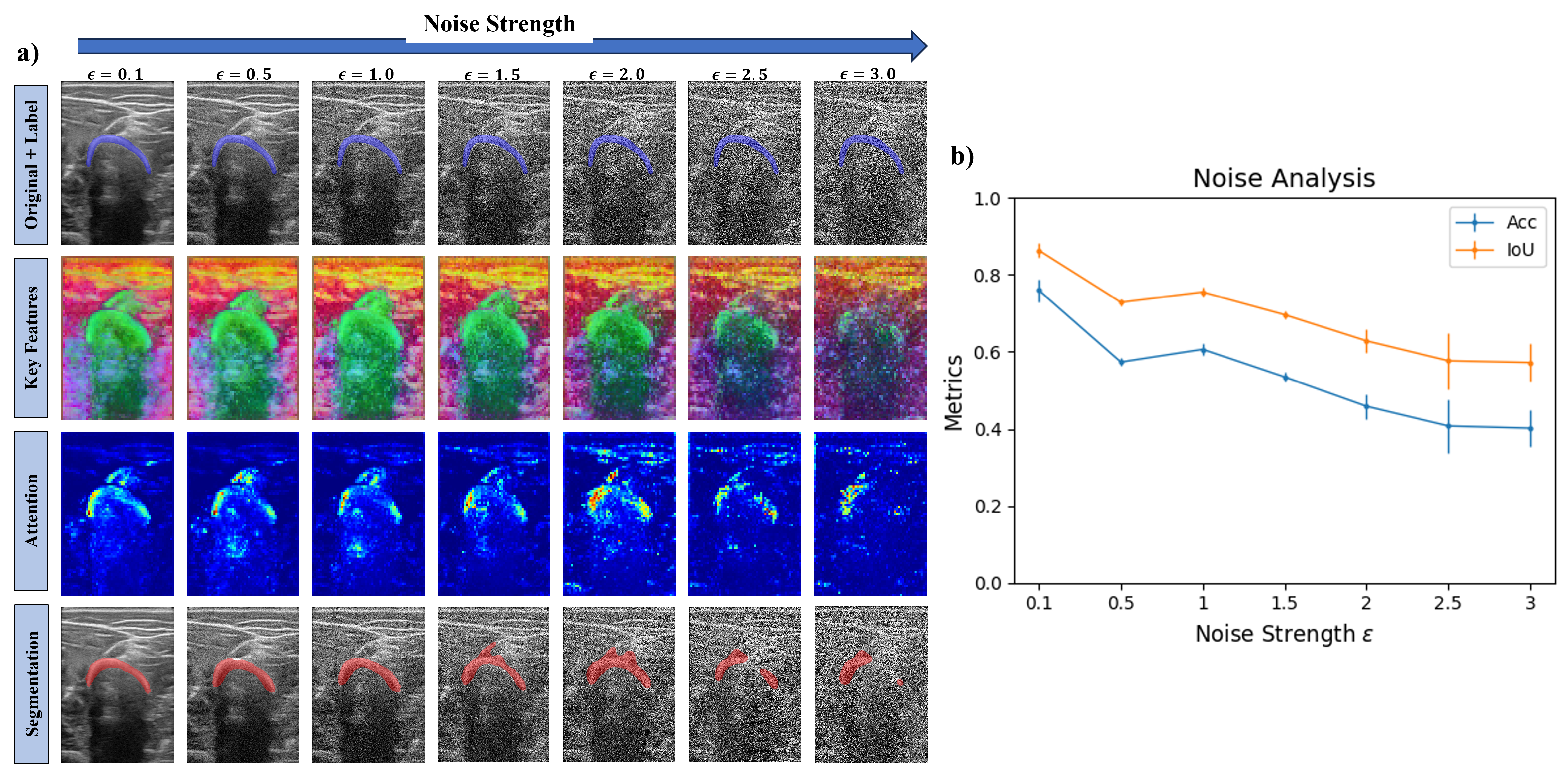
We further assessed DINO by introducing white noise to the dataset. Being an image \(\mathcal{I}\), the image input to DINO was \(\mathcal{I}_{\texttt{Noisy}} = \mathcal{I} + \epsilon \cdot \mathcal{N}(0, 1)\). We segmented five images from the domain Source 1 Arm Subject 1 and incrementally increased the white noise strength by tuning \(\epsilon\). We performed this last experiment to evaluate how the deep features and attention maps change as well as the resulting segmentation masks with increasing noise, gaining intuition on how robust DINO can be.

As observed in the following figure, the Keys features and the attention weights start being affected by the noise at \(\epsilon = 2.0\). Keys features are less efficient at describing the bone from the surrounding structures, and the attention maps start shifting the attention to only the left side of the bone and the muscle line above the bone. Segmentation results show that with increased noise, some parts of the muscle are segmented and for \(\epsilon \geq 2.5\), the right side of the bone is not included on the segmentation mask.

Taking a look at the metrics, the more the noise strength is increased, the lower the Dice and IoU values obtained. From little noise to the highest tested in this experiment, a reduction of about 50% for both Dice and IoU occurs.

Results with noisy images. a) Original, Keys features, attention, maps and segmentation results for different values of $\epsilon$. b) Dice and IoU metrics for different values of $\epsilon$.

Discussion

In this project, we used a DINO ViT model to segment bone heads from ultrasound images using a zero-shot methodology involving clustering. We first studied how the model deep features change across different layers, and chose Key features as the most appropriate for characterizing bone. We then segmented bone from different image domains, initially employing batches of images from the same domain, and then combining them. Finally, we tested DINO and its robustness by adding additional noise.

Encouraging results were found in the deep features of the model. We could appreciate how both Key and Query features were capable of differentiating bone, some muscle regions, and skin tissue. We also obtained surprisingly good segmentation masks for a zero-shot methodology on a new dataset as ultrasound b-mode images are. In particular, the image domain “source 1 arm subject 1” presented very similar segmentation masks compared to the labeled ones, giving an idea of how semantic features obtained by DINO extend beyond its training data domain, displaying astonishing generalization. Even when adding noise to the image dataset, DINO Key features kept describing the bone up to high noise strengths.

While the project has yielded promising results, there are several limitations to take into account. First, we should note that the success of the zero-shot methodology has relied on an initial hyperparameter tuning, finding the threshold \(\tau\), the voting percentage, and the number of clusters. However, we are aware that the optimal configuration may vary across different datasets or imaging conditions. Additionally, we focused on segmenting only bone, but we have not explored the capabilities of DINO to segment other tissues or structures. We acknowledge that a comprehensive medical imaging solution should combine the segmentation of multiple relevant structures for a general understanding and application. Finally, only two anatomical parts (arm and leg) and two subjects were included in the dataset. To better explore the applicability of the model, a more diverse dataset containing more anatomical parts from more subjects should be considered.

In conclusion, this project demonstrates the potential of employing the DINO ViT model for ultrasound bone segmentation using a zero-shot methodology. We believe that this work lays a foundation for future improvements, promoting a more comprehensive understanding of DINO’s capabilities in medical image segmentation.