Challenges in Deep Learning Surrogates for Constrained Linear Optimization
Learning a deep net to optimize an LP, based on predicting the optimal basis vector. Surveys existing approaches in the literature. Demonstrates high accuracy of feasibility and optimality on small problem instances, but documents issues when scaling to larger problems. Benchmarks against a modern optimization solver, with discussions on upfront training vs. variable inference computation times.
Introduction
Physics-informed machine learning has emerged as an important paradigm for safety-critical applications where certain constraints must be satisfied.
The goal of this project is to learn a deep learning surrogate for a linear programming optimization problem with hard constraints. The overall approach is inspired by standard KKT conditions. This project will attempt a different DNN approach that aims to predict basic feasible solutions (BFS), and then benchmark it against a modern optimization solver. This project will highlight challenges in designing deep learning LP surrogates.
Due to computing resource limits, the focus on the project will be more about broad training strategy choices (“discrete” architecture choices), instead of a systematic sweep of hyperparameters.
Optimization problem
We are interested in learning to optimize this linear program with $n$ variables and $m$ equality constraints:
\[\begin{aligned} \min \quad &c^T y \\ \text{s.t. } &Ay = b, (\lambda) \\ &x \geq 0 \end{aligned}\]The KKT conditions are:
\(\begin{aligned} \quad Ay &=b, \\ A^T\lambda + s &= c, \\ y_i s_i &= 0, \forall i \in [n], \\ y, s &\geq 0 \end{aligned}\)
Literature review
Fundamental connections between deep learning and the polyhedral theory central to optimization has been noted in
Previous literature on machine learning for linearly-constrained optimization problems could be categorized by how they manage the various components of the KKT conditions. In many of these papers, there is some common deep neural architecture at the start (e.g. FCNN or GNN); and then to attempt to recover a feasible solution, the final layers in the architecture correspond to some “repair” or “correction” layers that are informed by optimization theory.
(KKT equalities + Complementarity): Building on
(Primal equality + Subset of primal inequalities): E2ELR

Source:
(Primal equality + All primal inequalities): Following a similar application in control/RL,

Source:
Alternatively, “Deep Constraint Completion and Correction” DC3
To truly guarantee polyhedral constraints,
(Primal + dual approaches): Previous work
In a similar vein of trying to incorporate the whole primal-dual problem structure, the GNN for LP paper
Method
Data generation
Since the focus is on learning LP’s generally, the dataset is fully synthetic. For this project, focus on having matrix $A$ fixed (one was created with entries drawn from the standard normal distribution), and training over different data examples of $x=(b,c)$. As an application example, this can represent learning on a fixed electric grid network topology and technology set, but learning to predict over different RHS resource capacities / renewables availabilities, and different fuel costs.
To ensure feasibility (primal problem is feasible and bounded), the space of examples is generated by first creating primitive or latent variables, for each of the $N$ samples (this was implemented in PyTorch to be efficiently calculated in a vectorized way):
- Binary vector $\xi \in {0,1}^n$ representing the optimal LP basis, with $\sum_i \xi_i = m$; the value is drawn uniformly from the $(n \text{ C } m)$ possible combinations. Practically this was implemented as a batched permutation of an identity tensor with extra columns.
- Nonnegative vector $d \in \mathbb{R}^n$, with each $d \sim U[0,1]$ uniformly drawn to be nonnegative.
- Then for each element $i$, use $\xi_i$ to determine whether to assign the value of $d_i$ to either the primal variable $y_i$ or the dual slack variable $s_i$. This way complementary slackness is enforced. Namely,f \(\begin{aligned} y &:= d\odot\xi, \\ s &:= d\odot(1-\xi) \end{aligned}\)
- Sample $\lambda \in \mathbb{R}^n, \lambda_i \sim U[0,1]$.
- Finally construct $b=Ay, c= A^T\lambda + s
By constructing the dataset in this way, we also know the ground truth optimal solutions (which might not be unique if there are degenerate solutions, which is assumed here to have low impact due to the random coefficients), and importantly also the optimal LP basis.
Model
As a different approach, this project will try to predict the underlying latent target $\xi$, i.e. the optimal LP basis, as a classification problem. Since there may be non-local interactions between coefficients and variables, a fully-connected architecture is chosen, where every layer is followed by a ReLU nonlinearity. The neural net forms a mapping between inputs $x=(b,c) \in \mathbb{R}^{m+n}$ to outputs $\hat{\xi} = f(x) \in {0,1}^{m}$, i.e. binary classifications of whether each variable is chosen in the LP basis. Below is an illustration of all the LP bases vectors for the $n=10, m=5$ problem size; there are $10 \text{ C } 5 = 252$ bases.

Supervised vs. self-supervised learning: Many of the referenced papers devise self-supervised training methods, which is motivated by the expensive computational costs (time) to solve the dataset instances with traditional optimization solvers. However, this synthetic dataset is somewhat of an inverse-problem approach, i.e. by starting out with a sample of assumed optimal solutions, the optimal solutions are very efficiently identified during dataset generation. This synthetic generation can also be thought of as a data augmentation method.
Since this is binary classification, the training loss used will be binary cross entropy, which is defined in PyTorch for each sample as: \(l(\hat{\xi},\xi) = [l_1, ..., l_i, ..., l_n],\ \ l_i = \xi_i \log \hat{\xi}_i + (1-\xi_i) \log (1-\hat{\xi}_i)\)
A softmax layer multiplied by $m$ is optionally added at the output of the NN, to enforce the requirement that there should be $m$ basic variables (in a continuously-relaxed way).
Equality completion: Once this is done, the LP basis uniquely determines a basic solution (but not necessarily feasible) according to \(\hat{y}^* = (A^\xi)^{-1}b,\) where $A^\xi$ is the $m\times m$ submatrix corresponding to the chosen columns. Rather than matrix inversion, this can be solved in a batched way with PyTorch (torch.linalg.solve) to obtain all samples’ solutions. The entire flow, from supervised dataset generation to neural net prediction and then $y$ solution recovery, is illustrated in the flowchart below.

As baselines, also consider the DC3 model, where novelty versus the original paper is that here both $b$ and $c$ are varied across samples (as opposed to only the RHS $b$ vectors). Also benchmark against a modern first-order based optimization solver OSQP
All experiments are implemented on Google Colab T4 GPU instances (except OSQP which can use CPU). Neural network training is optimized with Adam.
Results
Approximation and generalization
Small scale ($n=4,m=2$)
On a small $n=4,m=2$ problem, the proposed method (using a 3-layer FCNN with width-100 hidden layers; and trained for $<$100 epochs) can achieve near-perfect accuracy ($>$0.997) in both training and testing. The training set has 10,000 samples, and the test set has 1,000 samples, both generated according to the method above. The learning rate used was $10^{-3}$.
The accuracies when including and excluding the softmax layer (sum to $m$) are reported in the plot below, where this layer does have some (very) small positive effect on training and testing accuracies. More importantly, the $\hat{\xi}$ predictions after the solution recovery step are all feasible, i.e. with no negative elements, and the predicted optimal solutions can be seen in the right plot to match extremely closely with the ground truth $y^*$. This latter property is a desirable feature of the proposed method, that is, once the correct basic feasible solution is predicted, then the linear equation solver will precisely recover the optimal solution.

Scaling up ($n=10,m=5$)
Scaling up to a still quite small problem size of $n=10,m=5$ (i.e. 6.25 times larger in terms of $A$ matrix entries), now encounters generalization issues. The same network parameter sizing and training scheme was used here. The left plot shows training accuracy reaches about 0.97 after 300 epochs (and should continue rising if allowed to continue). However, the testing accuracy plateaus at around 0.93 with no further improvement.
More importantly, while a $>$0.9 accuracy in deep learning tasks is often sufficient, in this particular context the inaccuracies can lead to optimization problem infeasibilities. This is seen in the right plot, where mis-classified $\hat{\xi}$ result in catastrophically wrong $\hat{y}$ primal solution predictions (the severe orange prediction errors in both negative and positive extremes); even when the remaining correctly-predicted $\hat{\xi}$ samples receive precisely correct solutions.

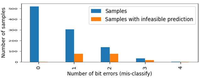
Furthermore, even though there are about $1-0.93 = 7%$ of individual $\xi_i$ entries that are mis-classified, these errors are fairly spread across various samples. This results in a $19%$ infeasibility rate in the test set, i.e. $19%$ of the predicted $\hat{y}$ vectors violate the nonnegative constraint. In other words, since this particular approach is predicting every individual entry of the basis vector, even small errors for each sample can lead to the overall prediction being wrong. This disproportionate impact is intuitively explained by examining the distribution of bit-wise errors plotted below. Most samples result in 0 bits of error, and then the remaining samples mostly get 1 or 2 bits of error. This means that errors are spread out among many samples, leading to a high rate of infeasible prediction vectors.

Attempts to improve accuracy
The previous training error plot appears to show an generalization or overfitting problem. Based on this, various data augmentation techniques were attempted, such as perturbing $b$, $c$, or both vectors (both based on random noise vectors and simple scaling invariance of $\alpha b, \beta c$ while keeping the latent $\xi$ targets; as well as generating new $\xi$ vectors after regular numbers of epochs; different schedules of the aforementioned were also tried. However, none of these attempted approaches were able to produce validation accuracy rates significantly above the original $\sim 0.93$.
Notably, an alternative architecture was tried: instead of outputting size-$n$ binary vectors, now try to predict multi-class classification out of the 252 basis vector classes. This actually resulted in worse testing set performance. Intuitively, treating all bases as discrete classes does not leverage the geometric proximity of 2 adjacent bases (e.g. which are off by 1 in Hamming distance).
Benchmarking
vs. DC3 (an “interior” learning approach)
As a comparison for the $n=4,m=2$ case, the DC3 methodology was implemented using a 3-layer neural net and the self-supervised training loss of the primal objective plus infeasibility penalty, with a chosen penalty rate of 10: \(\mathcal{L} = c^T \hat{y} + 10 ||\max\{0, -\hat{y}\}||^2_2\)
The number of inequality correction steps during training was chosen to be $t_{train} = 10$, and to maximize the chance of feasibility a very large $t_{test} = 10,000$ was used (i.e. allow many inequality-correction gradient steps during testing inference).

With a learning rate of $10^{-5}$, the training stabilizes after about 30 epochs. Overall, the predictions are fairly accurate in terms of the out-of-sample average objective: $-0.247$ (a 2% optimality gap versus the ground truth), and an $R^2$ of predicted objective values of 0.9992 (see middle plot). (The qualitative results were robust to faster learning rates too: A previous higher lr=$10^{-3}$ produced a tighter average objective gap, but the optimal solution deviation versus the ground truth was larger.)
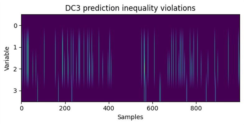
However, despite being designed to enforce all hard constraints, the predictions still resulted in infeasible negative values (see the negative dip in the right plot). A similar disproportionate classification error to infeasibility impact is seen here (albeit to a lesser extent): $2.6%$ of all output entries are negative, while $7%$ of test samples lead to an infeasible prediction.
Similarly to before, inequality violations are spread out among different samples, rather than all concentrated within a few samples; this is seen in the plot below. This provides an explanatory mechanism for the relatively large infeasible rate.

vs. Optimization solver
Thus far, the DNN is able to scale quite well along the number of samples dimension, but not the actual problem dimension (number of variables and constraints).
Return for now to the small $n=4,m=2$ case for which the DNN method achieves perfect out-of-sample testing accuracy. A next practical question is how does this method compare with “classical” optimization methods, or in what contexts would we prefer one over the other?
Note that there are only $4 \text{ C } 2 = 6$ bases. So once the NN produces a $\hat{\xi}$ estimate, these can be mapped to an index in ${1,2,…,6}$. All possible non-basic submatrix inverses can be pre-calculated. In total, to evaluate 1 million testing samples, the DNN predict-basis approach takes:
- 46 sec for training
- 0.002 sec for prediction of $10^6$ samples
- 10 sec to map $\xi$ to bases indices (note this is not done in a fully vectorized way and potentially could be sped up).
- $<0.001$ sec to batch matrix multiply every sample $j$’s: $(A^{\xi^j})^{-1}b^j$. Note this is done using einsum which is very efficient on CUDA.
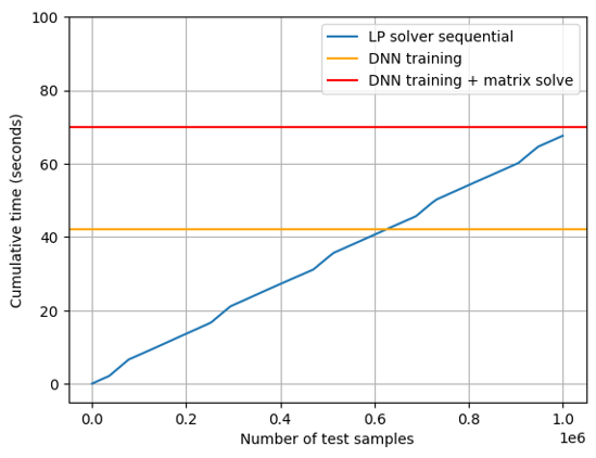
In comparison, even when running all the 1 million problem instances fully sequentially, the OSQP solver took a total of 67 sec, i.e. solving about 15,000 problem instances per second.
This means that this DNN model here only achieved a speedup factor of about 1.2x, when including the DNN training time. Furthermore, the above “mapping” step is a remaining coding bottleneck at DNN inference time, and this will scale linearly as the test sample size increases; i.e. this speedup ratio is unlikely to increase much beyond this at higher sample sizes.

The timing tradeoff can be understood in terms of fixed vs. variable costs, as plotted here. Note the orange and red lines, representing this project’s DNN approach, is using the batched matrix solve instead of the pre-computing 6 matrix inverses (thus taking longer in the solving stage). Despite its very large speedup when only considering the prediction step, holistically the DNN approach here did not pose very significant timing advantages over the optimization solver.
Conclusion
This project broadly compared 3 very different approaches to LP optimization: 1) a DNN to predict the optimal LP basis, 2) the DC3 method, and 3) optimization solver. Among the 2 deep learning methods, on the small $n=4,m=2$ problem, the LP basis method produced more robust and accurate results (i.e. it was able to perfeclty learn the input to optimal solution mapping, for the chosen data domain) compared to DC3 which already faces inequality violation issues. However, neither deep learning methods were able to easily scale to the slightly larger problem.
Qualitatively, the predict-LP-basis approach can result in “all-or-nothing” accuracy, i.e. predicting the correct basis vector results in the globally optimal solution, whereas even a nearby classification error can lead to catastrophic primal infeasibilities (due to enforcing the equality constraint). Moreover, in both predict-basis and DC3, inequality violations tend to be spread out among different samples, leading to disproportionate impact on the percentage of infeasible solution vector predictions.
Domain-specific knowledge and leveraging problem structure may be needed for tractable DNN solutions for LP optimization. This includes real-life choices of how much accuracy we need exactly in different aspects of the problem (e.g. different components of the KKT conditions).