Understanding Bias in Speech to Text Language Models

Do language models have biases that make them better for latin based languages like English? To find out, we generate a custom dataset to test how various language features, like silent letters, letter combinations, and letters out of order, affect how speech2text models learn and compare these results with models trained on real human language.

Motivation

With all the buzz that ChatGPT is getting recently, it is clear that machine learning models that can interact with humans in a natural manner can quite literally flip the world around. If that is not enough proof, Siri and Google Assistant, their popularity and convenience can give you a bit more of an idea. We can see how speech processing is important as a way for humans and computers to communicate with each other, and reach great levels of interactivity if done right. A lot of the world’s languages do not have written forms, and even those that do, typing can be less expressive and slower than speaking.

The core of these assistant systems is automatic speech recognition, often shortened as ASR or alternatively speech2text, which we will be using. This problem sounds rather simple: turn voice into text. However easy it might sound, speech2text is far from solved. There are so many factors that affect speech that makes it extremely difficult. First, how do we know when someone is speaking? Most speech2text models are trained on and perform well when the audio is clean, which means there is not a lot of noise. In the real world, however, one can be using speech2text in a concert or a cocktail party, and figuring out who is currently speaking to the system amid all the noise is a problem in itself! Another important factor that complicates speech2text is that we don’t all talk the same way. Pronunciations vary by person and region, and intonation and expressiveness change the acoustics of our speech. We can see this in full effect when auto-generated YouTube caption looks a bit.. wrong.

From https://www.reddit.com/r/funny/comments/ha7dva/youtube_auto_captions_spot_on/

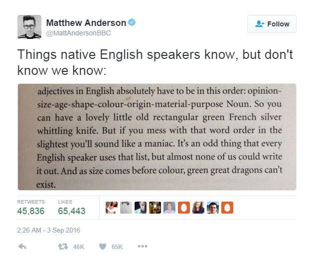
Aside from who and how we talk, another big part that makes speech2text hard has to do with the idiosyncrasies of text and languages itself! Some idiosyncrasies of language include orthography, the system of how we write sounds and words, and syntax, the system of how words string together into sentences. If you are familiar with English, you would be familiar with the English syntax: subject, verb, object, and a particular order for adjectives. We would instinctively say “small white car,” but not “white small car” and most definitely not “car white small.” Cross over the English channel to France (or the St. Lawrence River to Quebec), and the order changes. For French, you would say “petite voiture blanche,” which word for word is “small car white.”

Travel a bit further and you would see that Chinese uses “白色小车” (”white color small car”), Thai uses “รถสีขาวคันเล็ก” (”car color white * small”) and Kannada uses “ಸಣ್ಣ ಬಿಳಿ ಕಾರು” (”small white car”, same as English). Aside from order of adjectives, larger differences in syntax include having the subject appear first or last in a sentence, position of verbs, and how relative clauses work. All this means that language is quite non-linear, and natural language models that understand language must cope with our silly little arbitrary orders!

From https://www.bbc.com/news/blogs-trending-37285796

Thankfully though, for speech2text how sentences work is not as important as how phonetics and orthography works. But even then, things are not quite smooth sailing either. We sometimes take for granted how difficult reading is, perhaps until you start to learn a second language and realize how much we internalize. English is notorious for not spelling words the way it sounds, mostly because writing was standardized a long time ago and pronunciation has shifted since. This makes it difficult for machine learning models to try learn.

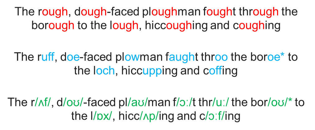
Sentence from https://en.wikipedia.org/wiki/Ough_(orthography)

Wow, look at all those words with “ough”! There are at least eight different pronunciations of the word, or from another point of perspective, at least eight different audios magically turn out to be spelt the same! In the diagram we tried substituting the red “ough”s to their rhymes in blue, keeping in mind that some dialects pronounce these words differently (especially for “borough”), and in green is the International Phonetic Alphabet representation of the sounds. IPA tries to be the standard of strictly representing sounds as symbols. What’s at play here? English is plagued with silent letters (”knight”), and extraneous letters (all the “ough”s and more).

Some languages are more straightforward in their orthography than others. Spanish tends to be fairly phonemic, which pretty much means that their writing and speaking are quite in sync. French, however, is very famous for its silent letters. A word like “hors-d’oeuvres”, which means appetizer, can be represented in IPA as [ɔʁ dœvʁ], you may see that around half the letters aren’t pronounced! Kannada, a language in South India that is spoken by one of our group members, is said to be quite phonemic, but doesn’t come without a different kind of headache. A number of languages, predominantly in South Asia and Southeast Asia, use a kind of writing system that combines a consonant character with a vowel character to form a new character that represents the consonant-vowel combination. The new character retains some part of the original consonant and vowel in some cute manner, kind of like the letter Æ but dialed up many notches. Most abugida systems descend from the 3rd century BCE Brahmi script.

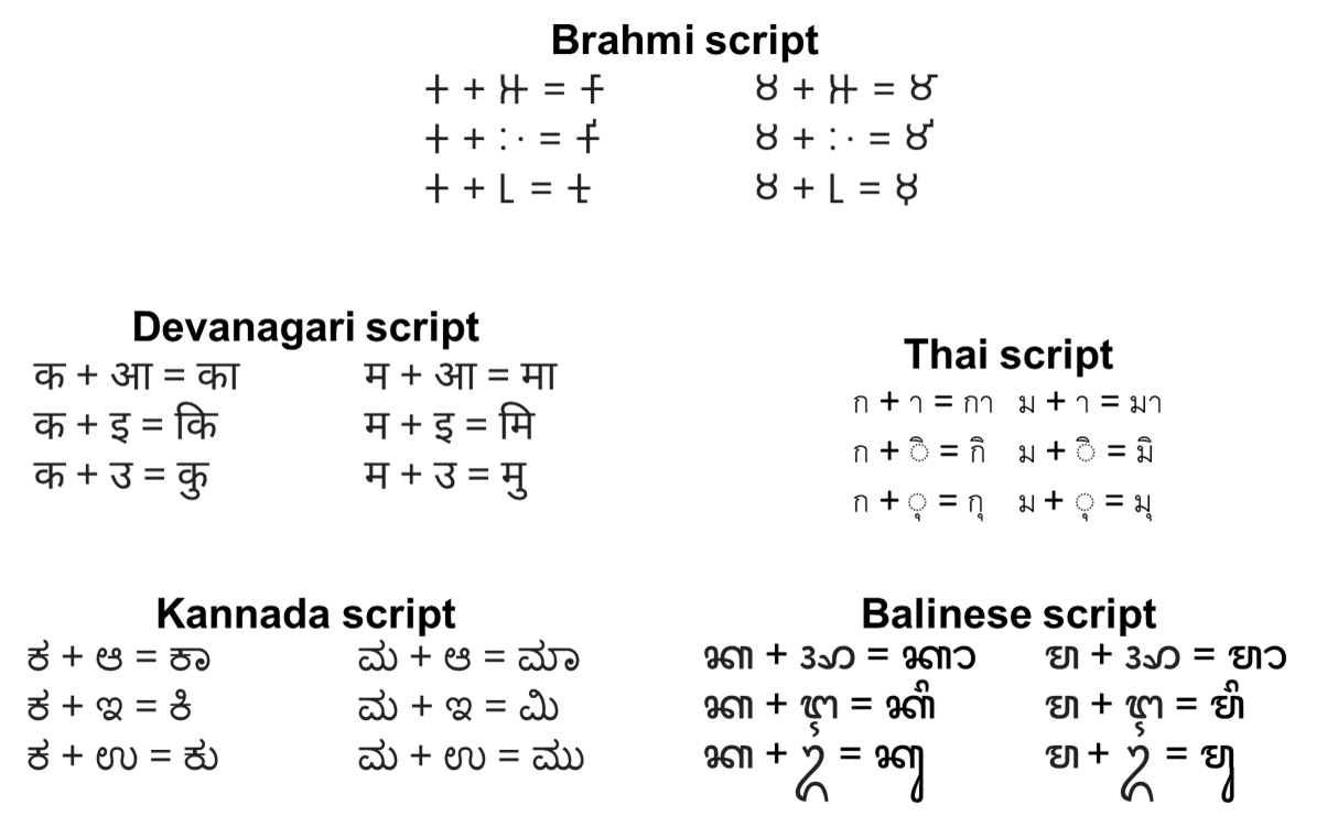
Above are some examples of scripts of this type, demonstrating two consonants k and m combining with vowels long a, i and u. Another interesting feature for some of these writing systems is that sometimes the vowels jump to the front, for example in Thai ก (k) + เ (e) = เก (ke). Again, writing is non-linear at times!

Past Work

Past work shows success in training speech2text models in German, Spanish, and French , . Some use pruning and finetuning of state of the art English models, and others train models from scratch for each language. Other works such as show that models can learn less common languages, like Thai which is the language our other group member speaks, as well, but they are more complex and specific to each language. circumvents this by pruning wav2seq (a SOTA speech2text model) and finetuning the model for different languages. While this showed promising results, we wanted to dive deeper to understand, from a linguistic and data driven perspective, the biases that simple speech2text models had.

Many state of the art models rely on encoder-decoder models. An encoder is used to create an expressive feature representation of the audio input data and a decoder maps these features to text tokens. Many speech models like , , also use self-supervised pretraining on the encoder for better performance. One example is the Wav2Seq. Wav2Seq uses unsupervised pretraining to annotate audio samples with unique characters in the form of a psuedo language. The building blocks for these encoders are generally transformer based .

Other methods use deep recurrent neural networks like in . RNNs are great at sequential tasks and have an internal memory to capture long term dependencies. Transformer based methods have outperformed RNNs and LSTM based architectures now though.

How do these features (idiosyncrasies) differ between languages and does this affect how well speech2text models learn? By doing more ablation studies on specific features, maybe this can inform the way we prune, or choose architecture, and can also help determine the simplest features necessary in a speech2text model that can still perform well on various languages.

There has been work that perform ablation studies on BERT to provide insight on what different layers of the model is learning . Experiments suggest lower layers learn phrase-level information, middle layers learn syntactic information, and upper layers learn more semantic features. We want to do a similar study, but on dissecting the components of language rather than the components of a particular SOTA model. Our hypothesis is that by doing so, we can be better informed when selecting preprocessing methods and models.

Let’s get started with some experiments!

Generating a Dataset

We want to explore how each of these language features affects how speech2text models learn. Let’s create a custom dataset where we can implement each of these language rules in isolation. To do that, we’ll build out our own language. Sounds daunting — but there are only a key few building blocks that matter to us. Languages are made of sentences, sentences are made of words, words are made of letters, and letters are either consonants or vowels. Let’s start with that.

From , languages have 22 consonants on average and about 9 vowels on average so that’s what we’ll have in our language too. We represent consonants as positive integers from 1 to 23 and vowels as negative integers from -9 to -1. After all, letters are just symbols!

A word, at it’s most crude representation, is just a string of these consonants and vowels at some random length. To make sentences, we just string these words together with spaces, represented by 0, together.

Here’s a sample sentence in our language:

[14 -2 -9 13  0  8 16 -8 -2  0 -3 -8 16 12  0 10 20 -3 -7  0 14 18 -9 -4
  0 16 -3 -5 14  0 -3  9 -8  3  0 -9 -1 22  7  0 12 -5  6 -7  0 -7 22 12
 -2  0 22 -9  2 -2  0 17 -2 -8  9  0  1 -4 18 -9  0 19 -7 20 -2  0  8 18
 -4 -2  0 -9  8 -4 15  0 -9 -2 22 18]

Ok, that seems a little meaningless. We don’t have to worry about meaning in the general semantic sense though. What we do care about, is pronouncing this language, and creating a mapping from these written sentences to an audio sample. Let’s do that next. Audio samples can be represented as spectrograms. Spectrograms give us a visual representation of audio by plotting the frequencies that make up an audio sample.

Here’s an example:

When we say “It’s never too early to play Christmas music”, this is what it might look like visually:

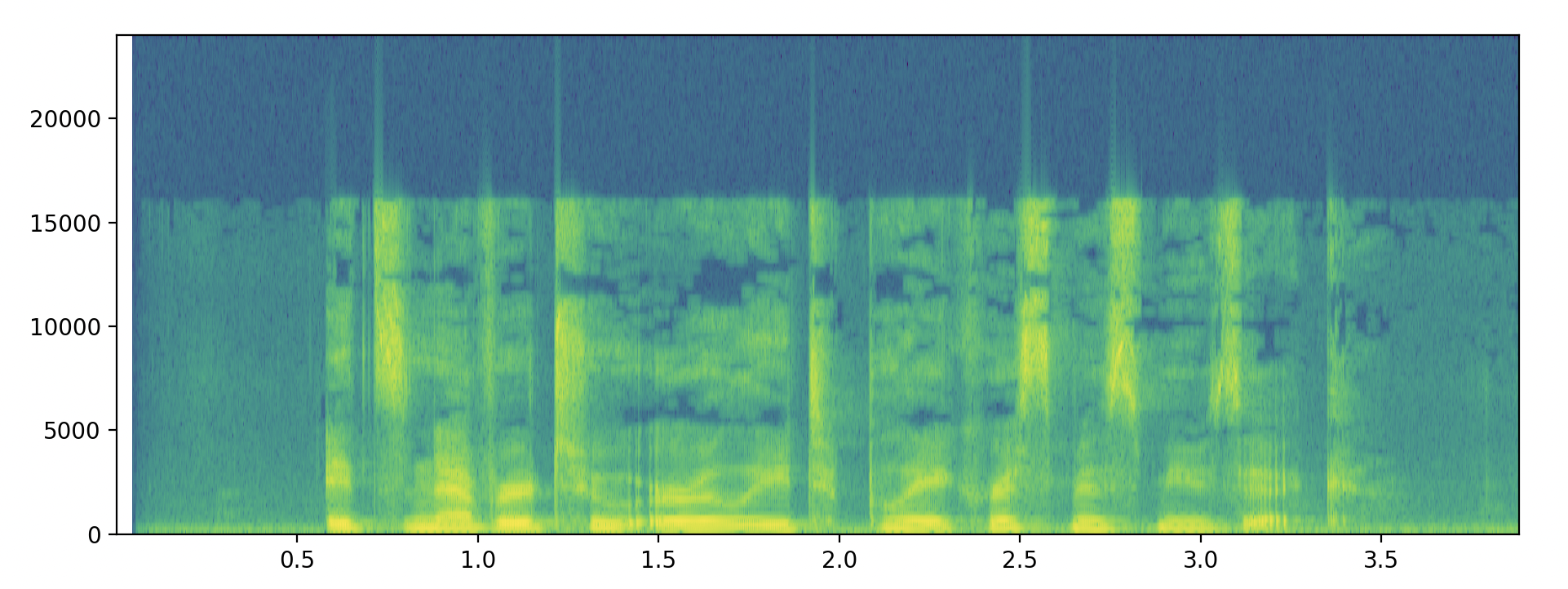
The key here is that we don’t exactly need audio samples, but rather an embedding that represents an audio sample for a written sentence. Embeddings are just low dimensional mappings that represent high dimensional data.

So, in our case, our spectrogram for a generated audio sample looks something like:

Even though audio samples might be complicated waveforms, the embedding for the first letter looks something like:

tensor([[ 3.6887e-01, -9.6675e-01,  3.2892e-01, -1.2369e+00,  1.4908e+00,
          8.1835e-01, -1.1171e+00, -1.9989e-01,  3.5697e-01, -1.2377e+00,
          4.6225e-01, -6.7818e-01, -8.2602e-01]])

Again, maybe meaningless to us who haven’t really learned this new language. There are some vertical columns of the same color, and these represent the silences between each word. You might notice that these columns aren’t exactly the same color, and that’s because we’ve added a bit of Gaussian noise to the audio embedding samples to simulate noise that might occur when recording audio samples on a microphone.

Ok great! We’ve got this perfect language that maps the same sentence to the same audio sample. Now, let’s get to work adding some features that we talked about in the previous section to make this language a bit more complicated.

We narrow our feature selection to the following three:

Silent Letters: letters in the written language that don’t appear in the phonetic pronunciation
Letter Combos: two letters combine in the script but are still pronounced separately
Letters out of Order: phonetic pronunciation is in a different order than written language

Silent Letters

Silent letters mean they appear in our written labels but not in our audio samples. We could just remove letters from our audio embeddings, but that’s a little funky. We don’t usually pause when we come to a silent letter — saying (pause - nite) instead of just (nite) for night. To preserve this, let’s instead add letters to our written label.

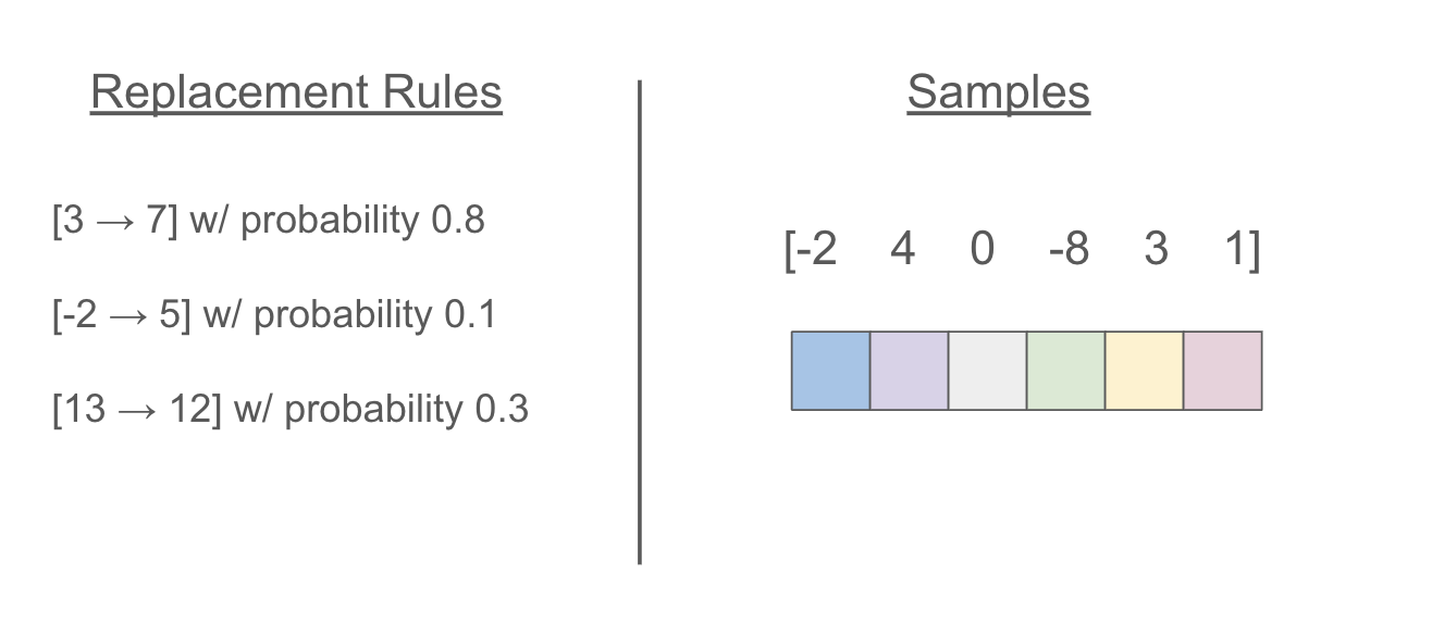
In the diagram above, we have a small written sample and some audio embeddings represented as colored blocks. We generate some rules similar to those on the left.

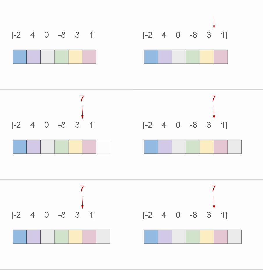
In this case, we add a 7 after the 3, simulating a silent letter at consonant 7. We then pad the audio sample with a silent (0) to make up for the size increase of the written label. Note that silent letters don’t add pauses during the audio.

Combining Letters

When combining letters, our written script changes, but our audio remains the same. We choose to combine every pair where a vowel follows a consonant. This is the most common case of letter combination in languages that have this feature.

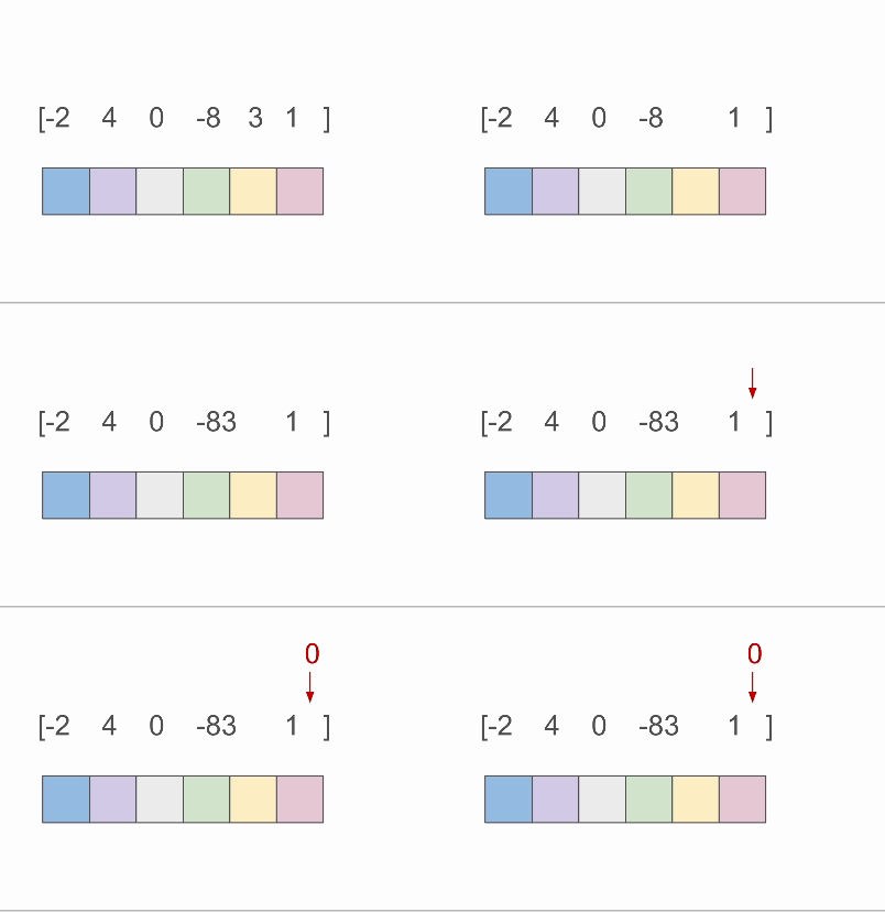
Here we have to pad the written labels as we combine two letters into one.

Letters out of Order

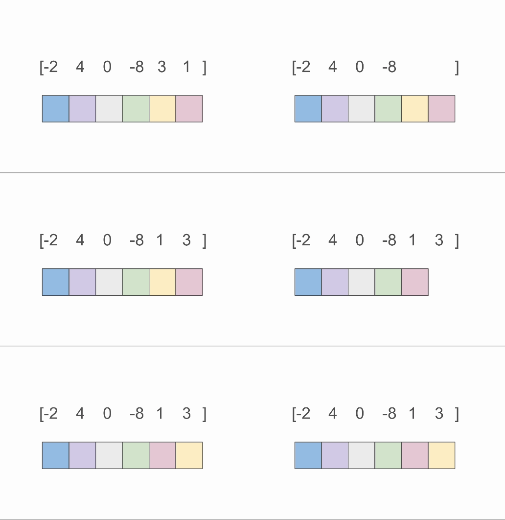
We choose some pairs of consonant and vowels. Swap the pair order for every instance of the pair in the written sample. No padding needs to be added here.

Controlled Experiments

Now for the fun part! Let’s see what happens when we test our new language, which each of these rules in isolation, with some models. Regardless of the model we choose, our goal is to learn a written label for a given audio sample.

We’re going to test our language with the building blocks of these state of art models — transformers and RNN. The results from these experiments can inform us on the biases that these fundamental models might have in their most “vanilla” state.

We hypothesize that transformers will perform better because RNN’s have a limited memory size, while Transformers use attention which means they can learn orderings from anywhere in the audio sample.

Results

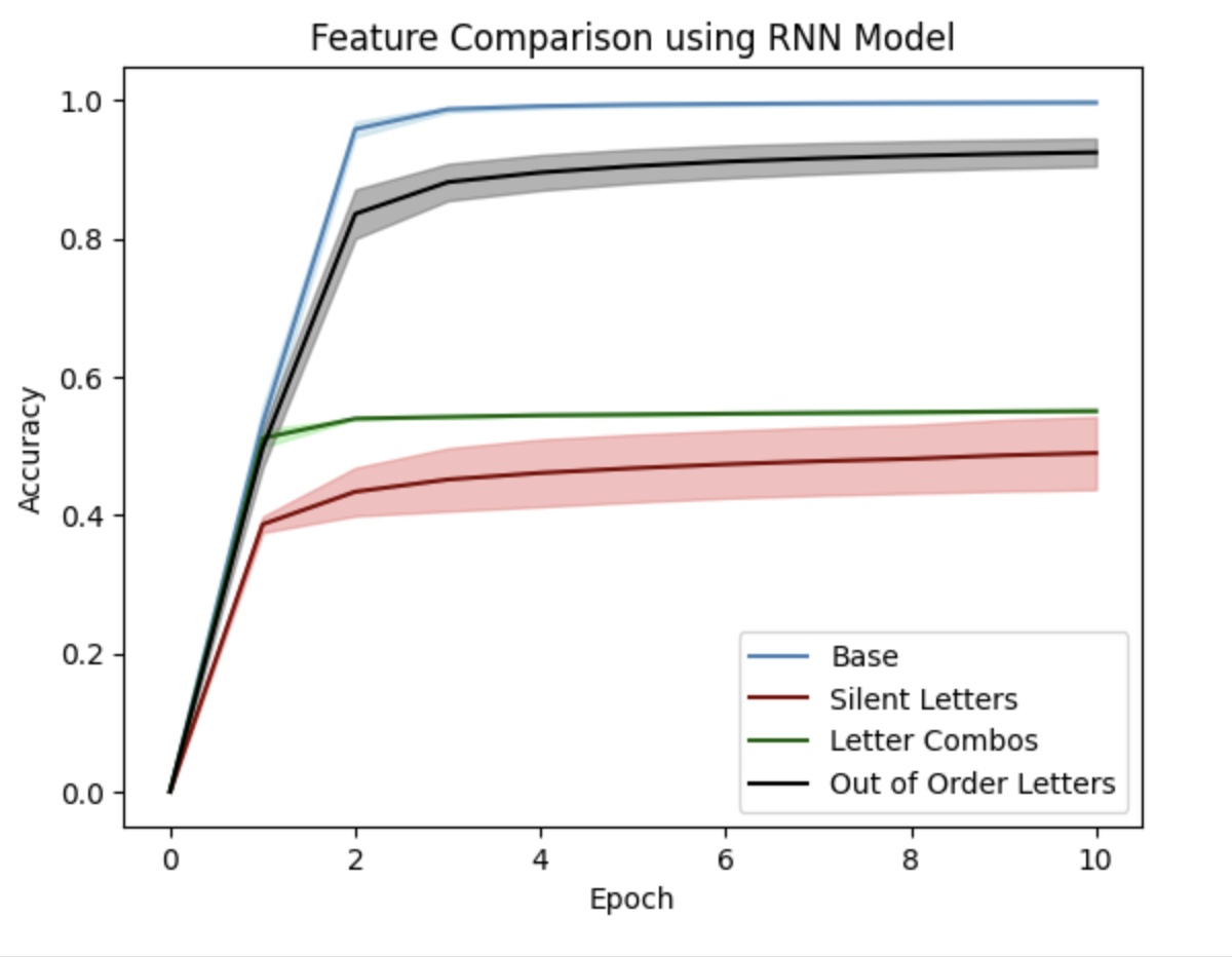
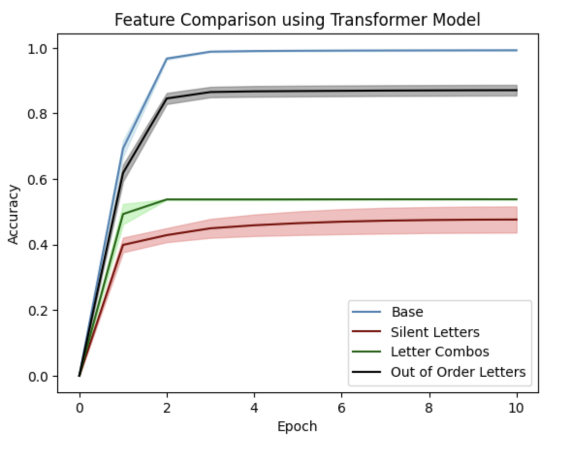
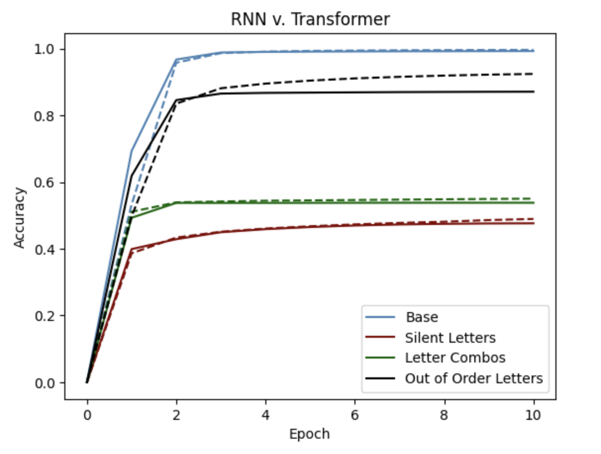
RNNs are dashed lines, Transformers are solid lines

Hmm..so Transformers performed better, but not that much better than our RNNs. This could be because our hypothesis that attention is better for long sequences and RNNs have limited memory may not apply. When we generated our language, the consonant and vowel orderings were pretty random. Our rules have some pattern to them, but not as much as a real human language — so maybe attention can exploit these better in real human language, but doesn’t give as much of an advantage in our generated dataset.

As for our features, it seems that silent letters perform significantly worse than some of the other rules. This makes sense because, attention and internal memory perhaps, provides some mechanism for dealing with swapping or out of order. Transformers have the ability to “focus” on features of the sample that it is deemed important. Our rules do have some pattern, and the models just have to learn these patterns.

With silent letters, though there is a pattern to an audio sample not being present, the rest of the sounds succeeding the silent letters are all shifted over. This is probably why letter combos also doesn’t do too great. With letter combos and silent letters, the one-to-one mapping between a letter and it’s phonetic pronunciation (or audio embedding) is thrown off for the rest of the sequence.

Corners Cut

This certainly tells us a lot! But, we should take these results with a grain of salt. There are some discrepancies with human language and the way that we generated our dataset that we should consider.

Actual audio speech recognition systems mostly don’t predict letter by letter, some do subwords and others do word level recognition; but in the grand scheme of things these distinctions may be negligible — after all, they’re all units! This means our controlled experiment, for our purposes, simulates character recognition models which may misspell words (”helouw” instead of “hello”). If the model is at the subword level, misspellings may decrease, since character sequences like “ouw” would not be in the list of possible subwords, or the vocabulary. “ouw” is a very un-English sequence, see if you can find a word that contains these three letters in succession! Misspellings like “hellow” might still happen though, since it is a plausible combination of English-like sequences “hel” and “low”. If the model is at the word level, there will not be misspellings at all.
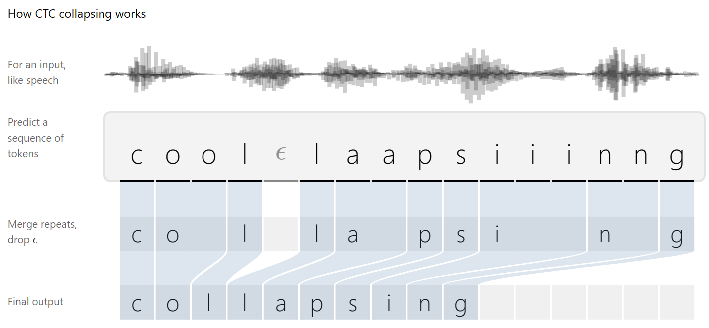
speech2text models generally either do encoder-decoder model, or otherwise typically the input and output do not have to match in dimension. Both options mean that there is no need to pad written or audio samples to make sure they’re the same length. In our case, we have to pad our written/audio to make sure everything is the same size. Connectionist Temporal Classification is used to postprocess outputs and compute loss.
- The way CTC works is that first it assumes that a letter may take more than one audio frame to say, which tends to be the case, especially for vowel sounds which are typically looooooooooonger than consonant sounds. There is also a special character epsilon that serves as the “character boundary” symbol, but is different from the silent symbol. The output of a CTC model is deduplicated, and epsilons are removed. Here is CTC in action from :

An effect of the letter combination script in our controlled experiment is that there will be some letter combinations that exist as a class (aka in the alphabet) but never seen in the dataset. For example (1, 12) are in the alphabet as consonants, but 112 isn’t a letter.
Actual language has tone, intonation, speed and noise that can make it harder to learn. Here is where something like Wave2Seq can help as tokens are clustered, so if someone takes a little longer to say AA, it will still register as the same pseudo token.

Real Language

Alas, real-world languages are more complicated than our controlled languages. We wanted to see if the patterns we learnt in our controlled experiments would still hold true for actual datasets. For this, we needed to find a relatively phonemic language and another language that differs only by one feature. As mentioned earlier, Spanish qualifies for the former, and French qualifies for the latter. French, to the best of our knowledge, is prevalent with silent letters, but don’t really exhibit other features in our controlled experiments.

We’re using the CommonVoice dataset, which is a crowdsourced dataset of people reading sentences in many languages, and might be harder to train because of how unclean the dataset as a whole may be. We preprocess the audio using a standard method, which is the following:

First, calculate the audio spectrogram and condense the result by summing up the amplitudes of a few frequencies that belong in the same “bucket”, to yield Mel-frequency cepstral coefficients (MFCC)
To add some temporal context, the differential of the MFCC and its second-degree differential are calculated and concatenated to the MFCC
The label vocabulary is constructed, by looking at what letters exist in the dataset, and the written data is converted to numbers

Behold, an example of the preprocessed dataset for Spanish!

target tensor: [30, 43,  1, 41, 53, 40, 56, 39,  1, 59, 52, 39,  1, 58, 39, 56, 47, 44,
        39,  1, 42, 43,  1, 43, 52, 58, 56, 39, 42, 39,  7]
target sequence: Se cobra una tarifa de entrada.

We tried training transformers and RNNs, with and without CTC, on this real-world data. Without CTC, the performances of the models are, respectfully, really bad. After a number of epochs, the only thing learnt is that the space character exists, and the 6% accuracy comes from the model predicting only spaces:

predicted tensor: [16 39  1  1  1  1  1  1  1  1  1  1  1  1  1  1  1  1  1  1  1  1  1  1
   1  1  1  1  1  1  1  1  1  1  1  1  1  1  1  1  1  1  1  1  1  1  1  1
   1  1  1  1  1  1  1  1  1  1  1  1  1  1  1  1  1  1  1  1  1  1  1  1
   1  1  1  1  1  1  1  1  1  1  1  1  1  1  1  1  1  1  1  1  1  1  1  1
   1  1  1  1  1  1  1  1  1  1  1  1  1  1  1  1  1  1  1  1  1  1  1  1
   1  1  1  1  1  1  1  1  1  1  1  1  1  1  1  1  1  1  1  1  1  1  1  1
   1  1  1  1  1  1  1  1  1  1  1  1  1  1  1  1  1  1  1  1  1  1  1  1
   1  1  1  1  1  1  1  1  1  1  1  1  1  1  1  1  1  1  1  1  1  1  1  1
   1  1  1  1  1  1  1  1  1  1  1  1  1  1  1  1  1  1  1  1  1  1  1  1
   1  1  1  1  1  1  1  1  1  1  1  1  1  1  1  1  1  1  1  1  1  1  1  1
   1  1  1  1  1  1  1  1  1  1  1  1  1  1  1  1  1  1  1  1  1  1  1  1
   1  1  1  1  1  1  1  1  1  1  1  1  1  1  1  1  1  1  1  1  1  1  1  1
   1  1  1  1  1  1  1  1  1  1  1  1  1  1  1  1  1  1  1  1  1  1  1  1
   1  1  1  1  1  1  1  1  1  1  1  1  1  1  1  1  1  1  1  1  1  1  1  1
   1  1  1  1  1  1  1  1  1  1  1  1  1  1  1  1  1  1  1  1  1  1  1  1
   1  1  1  1  1  1  1  1  1  1  1  1  1  1  1  1  1  1  1  1  1  1  1  1
   1  1  1  1  1  1  1  1  1  1  1  1  1  1  1  1  1  1  1  1  1  1  1  1
   1  1  1  1  1  1  1  1  1  1  1  1  1  1  1  1  1  1  1  1  1  1  1  1
   1  1  1  1  1  1  1  1  1  1  1  1  1  1  1  1  1  1  1  1  1  1  1  1
   1  1  1  1  1  1  1  1  1  1  1  1  1  1  1  1  1  1  1  1  1  1  1  1
   1  1  1  1  1  1  1  1  1  1  1  1  1  1  1  1  1  1  1  1  1  1  1  1
   1  1  1  1  1  1  1  1  1  1  1  1  1  1  1  1  1  1  1  1  1  1  1  1
   1  1  1  1  1  1  1  1  1  1  1  1  1  1  1  1  1  1  1  1  1  1  1  1
   1  1  1  1]
predicted sequence: Ea
target tensor: [71, 28, 59, 83,  1, 53, 57,  1, 54, 39, 56, 43, 41, 43, 11,  1, 36,  1,
        56, 43, 57, 54, 53, 52, 42, 47, 43, 52, 42, 53,  1, 43, 50, 50, 53, 57,
         5,  1, 42, 47, 48, 43, 56, 53, 52,  8,  1, 14, 59, 50, 54, 39, 42, 53,
         1, 43, 57,  1, 42, 43,  1, 51, 59, 43, 56, 58, 43,  7,  0,  0,  0,  0,
         0,  0,  0,  0,  0,  0,  0,  0,  0,  0,  0,  0,  0,  0,  0,  0,  0,  0,
         0,  0,  0,  0,  0,  0,  0,  0,  0,  0,  0,  0,  0,  0,  0,  0,  0,  0,
         0,  0,  0,  0,  0,  0,  0,  0,  0,  0,  0,  0,  0,  0,  0,  0,  0,  0,
         0,  0,  0,  0,  0,  0,  0,  0,  0,  0,  0,  0,  0,  0,  0,  0,  0,  0,
         0,  0,  0,  0,  0,  0,  0,  0,  0,  0,  0,  0,  0,  0,  0,  0,  0,  0,
         0,  0,  0,  0,  0,  0,  0,  0,  0,  0,  0,  0,  0,  0,  0,  0,  0,  0,
         0,  0,  0,  0,  0,  0,  0,  0,  0,  0,  0,  0,  0,  0,  0,  0,  0,  0,
         0,  0,  0,  0,  0,  0,  0,  0,  0,  0,  0,  0,  0,  0,  0,  0,  0,  0,
         0,  0,  0,  0,  0,  0,  0,  0,  0,  0,  0,  0,  0,  0,  0,  0,  0,  0,
         0,  0,  0,  0,  0,  0,  0,  0,  0,  0,  0,  0,  0,  0,  0,  0,  0,  0,
         0,  0,  0,  0,  0,  0,  0,  0,  0,  0,  0,  0,  0,  0,  0,  0,  0,  0,
         0,  0,  0,  0,  0,  0,  0,  0,  0,  0,  0,  0,  0,  0,  0,  0,  0,  0,
         0,  0,  0,  0,  0,  0,  0,  0,  0,  0,  0,  0,  0,  0,  0,  0,  0,  0,
         0,  0,  0,  0,  0,  0,  0,  0,  0,  0,  0,  0,  0,  0,  0,  0,  0,  0,
         0,  0,  0,  0,  0,  0,  0,  0,  0,  0,  0,  0,  0,  0,  0,  0,  0,  0,
         0,  0,  0,  0,  0,  0,  0,  0,  0,  0,  0,  0,  0,  0,  0,  0,  0,  0,
         0,  0,  0,  0,  0,  0,  0,  0,  0,  0,  0,  0,  0,  0,  0,  0,  0,  0,
         0,  0,  0,  0,  0,  0,  0,  0,  0,  0,  0,  0,  0,  0,  0,  0,  0,  0,
         0,  0,  0,  0,  0,  0,  0,  0,  0,  0,  0,  0,  0,  0,  0,  0,  0,  0,
         0,  0,  0,  0,  0,  0,  0,  0,  0,  0,  0,  0,  0,  0,  0,  0,  0,  0,
         0,  0,  0,  0,  0,  0,  0,  0,  0,  0,  0,  0,  0,  0,  0,  0,  0,  0,
         0,  0,  0,  0,  0,  0,  0,  0,  0,  0,  0,  0,  0,  0,  0,  0,  0,  0,
         0,  0,  0,  0,  0,  0,  0,  0,  0,  0,  0,  0,  0,  0,  0,  0,  0,  0,
         0,  0,  0,  0,  0,  0,  0,  0,  0,  0,  0,  0,  0,  0,  0,  0,  0,  0,
         0,  0,  0,  0,  0,  0,  0,  0,  0,  0,  0,  0,  0,  0,  0,  0,  0,  0,
         0,  0,  0,  0,  0,  0,  0,  0,  0,  0,  0,  0,  0,  0,  0,  0,  0,  0,
         0,  0,  0,  0,  0,  0,  0,  0,  0,  0,  0,  0,  0,  0,  0,  0]
target sequence: ¿Qué os parece? Y respondiendo ellos, dijeron: Culpado es de muerte.

Got it. Like our silent letter controlled experiment, a high mismatch between the audio frame and its written frame causes models to not be able to learn well. Let’s put in our mighty CTC Loss and see how it works! It turns out that after some 30 epochs, it still isn’t doing quite so well. Here, let’s see an example of a transformer trained on the Spanish dataset with CTC:

predicted tensor: [ 0 39  0 57  0 54 39  0 41  0 41  0 43  0 47  0 43  0 57  0 53  0 42  0
 58  0 47  0 53  0 41  0 54  0 39  0 43  0 57  0 43  0]
predicted sequence: aspacceiesodtiocpaese
target tensor: [71 28 59 83  1 53 57  1 54 39 56 43 41 43 11  1 36  1 56 43 57 54 53 52
 42 47 43 52 42 53  1 43 50 53 57  5  1 42 47 48 43 56 53 52  8  1 14 59
 50 54 39 42 53  1 43 57  1 42 43  1 51 59 43 56 58 43  7]
target sequence: ¿Qué os parece? Y respondiendo elos, dijeron: Culpado es de muerte.

Perhaps the transformer is too big for this and learns pretty slowly. It is starting to pick up on some sounds, for example for “¿Qué os parece?” it seems to have picked up “as pacce” and “respondiendo” has some similarities to “esodtio,” but we really needed to squint to see that similarity. If we let it run for longer, perhaps it would get better… slowly.

RNNs, however, came up on top. We’re using bidirectional LSTM RNN for this, and it seems that CTC works! Here’s the RNN trained on the Spanish dataset with CTC:

predicted tensor: [30  0 59  0 52  0 53  0 51  0 40  0 56 43  0 57  0 43  0  1 42  0 43  0
 42  0 47  0 42  0 39  0 42  0 43  0  1  0 89  0 51  0 40  0 43  0 58  0
 39  0 59  0 52  0 53  0  1 42  0 43  0  1 50  0 39  0  1  0 57  0 54  0
 39  0 88  0 53  0 52  0 39  0  7]
predicted sequence: Sunombrese dedidade ómbetauno de la spañona.
target tensor: [30 59  1 52 53 51 40 56 43  1 57 43  1 42 43 56 47 60 39  1 42 43 50  1
 52 53 51 40 56 43  1 58 39 86 52 53  1 42 43  1 23 39  1 16 57 54 39 88
 53 50 39  7]
target sequence: Su nombre se deriva del nombre taíno de La Española.

Looks great! Of course there are some word boundary mistakes, but overall it looks pretty similar. What about French? Here are transformer and RNN results for what we hypothesized is a language full of silent letter features:

predicted tensor (Transformer): [21  0]
predicted sequence (Transformer): L
predicted tensor (RNN): [18  0 47  0  1  0 56  0 56 40  0 54  0 44  0  1 55  0 40  0 55  1 53  0
 40  0 36  0 48 40  0 49 55  0 44  0 55  0 53 40  0 36  0 49  0  1 49 50
  0 53  0  1  0  1 44  0 47  0  1 40  0  1 51  0 50  0 55  0 36  0 49  0
  1 54  0 40  0 47 40  0 48 40  0 49 55  0  1 71  0  1 57  0 36  0 54  0
 44  0 54  6]
predicted sequence (RNN): Il uuesi tet reamentitrean nor  il e potan selement à vasis.

target tensor: [18 47  1 36  1 36 56 54 44  1 75 55 75  1 53 75 38 40 48 40 49 55  1 44
 49 55 53 50 39 56 44 55  1 40 49  1 14 56 53 50 51 40  1 50 82  1 44 47
  1 40 54 55  1 51 50 55 40 49 55 44 40 47 40 48 40 49 55  1 44 49 57 36
 54 44 41  6]
target sequence: Il a ausi été récement introduit en Europe où il est potentielement invasif.

Wow! The transformer got stuck in the blank hole black hole, but the RNN looks not too shabby. Some word boundary issues for sure, but we can see similarities. “potan selement” and “potentielement” actually do sound similar, as do “à vasis” and “invasif.” Definitely not as good as Spanish though. Here’s a comparison of losses for the four models:

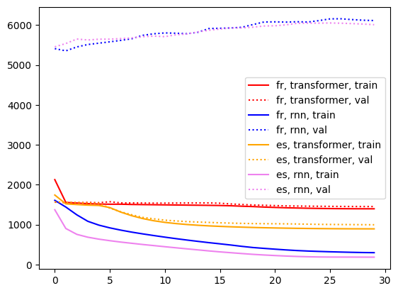
One thing that’s very much worth noticing is that the validation losses plateaued or rose during training. Did we overfit our data, or are these languages too hard that they can’t be fully learnt from our data, and the high loss is due to the idiosyncrasies of language? Probably both!

Now did these real-world explorations match our hypotheses from controlled experiments or not? Our hypothesis from controlled experiments says that French would do worse than Spanish, which is what we’re seeing. Additionally, we see a pretty significant gap in loss between transformers and RNN models, given that CTC loss is used.

Here comes the confusing part. Most literature would say that transformers should perform better than RNN, even with CTC. This matches with our controlled experiments but did not match our real-world experiments. What went wrong? For one, we think that our models might still be too small and not representative of actual real-world models. We also trained the models for quite a short amount of time with a small amount of data that might be noisy. Perhaps our recipe was just the perfect storm to cause our transformer model to be stuck in the blank hole. We found an article that documents the tendency for MLPs to get stuck in a stage of predicting blanks before moving on to predicting real characters, which sounds like what’s going on for us. Some other sources point to the assertion that input spectrogram lengths must be longer than label lengths, and suggest refraining from padding labels with blanks. We followed their suggestions but unfortunately could not bring the transformer models out of the blank hole.

Learnings

What have we looked at?

Linguistics: we learnt how weird languages can be!
Models: we touched upon how speech2text models usually work
Hindrances: we hypothesized and tested a few features that affected model performance
- Silent letters are our biggest enemies, followed by letter combinations and out-of-order letters
Battle: we compared how two different foundational models for speech2text against each other
- In our controlled experiments, it’s a pretty close call but transformer came up on top by just a slight margin
Real: we presented what a real-world dataset looks like, the data preprocessing methods, and checked if our learnings from controlled experiments hold
- Creating a spectrogram and a character vocabulary is the standard!
- French (silent letter-ish) vs. Spanish (perfect-ish) matches our hypothesis!
- CTC is the cherry on top for success but only works well with RNN, putting RNN on top by a long shot this time!

We would like to expand our linguistics experiments further as future work, as there are many more features and combinations not explored here (for example, Arabic writing usually drops all vowels — we imagine that this feature would affect performance a lot!) Another avenue of further work is to try train on other real-world languages to see whether our hypotheses still hold true.