Iterated Representation Learning
Representation learning is a subfield of deep learning focused on learning meaningful lower-dimensional embeddings of input data, and rapidly emerging to popularity for its efficacy with generative models. However, most representation learning techniques, such as autoencoders and variational autoencoders, learn only one embedding from the input data, which is then used to either reconstruct the original data or generate new samples. This project seeks to study the utility of a proposed iterated representation learning framework, which repeatedly trains new latent space embeddings based on the data outputted from the last round of representation. In particular, we seek to examine whether the performance of this iterated approach on a model and input dataset are indicative of any robustness qualities of the model and latent embedding space, and potentially derive a new framework for evaluating representation stability.
Introduction
Representation learning has become a transformative subfield of deep learning within recent years, garnering widespread attention for its sophistication in learning lower-dimensional embeddings of data beyond classical techniques such as principal component analysis (PCA). From class, we learned that desirable characteristics of good representations include minimality, sufficiency, disentangelement, and interpretability. However, because typical representation learning techniques such as autoencoders learn only one latent embedding from the input data, there exists a gap in the literature on the stability of the model and learned embeddings.
In this project, we thus explore a new approach to traditional representation learning techniques, in which embeddings for a given set of data are learned repeatedly until some sort of convergence with respect to the model and learned embedding space, a process we call Iterated Representation Learning (IRL); by analyzing the performance of this iterative approach, our work aims to discover potential insights into the robustness qualities inherent to a model and its associated latent embedding space. We propose an algorithmic framework for IRL, provide an empirical case study of the efficacy of our IRL framework on the MNIST dataset, and suggest a novel evaluation procedure for representation stability and robustness via iterated learning.
Representation Learning Primer
The goal of representation learning is to build models that effectively learn meaningful representations of the data. Representations are important for a variety of reasons, including determining which features are the most explanatory or variable in a dataset, compressing repeated information from a dataset to make it more compact, and learning more effective neural networks, to name a few examples. These representations are typically abstract and less interpretable than the input data, but of lower dimension, which makes them useful in capturing the most essential or compressed characteristics of the data.
More formally, representation learning aims to learn a mapping from datapoints \(\mathbf{x} \in \mathcal{X}\) to a (typically lower-dimensional) representation \(\mathbf{z} \in \mathcal{Z}\); we call this mapping an encoding, and the learned encoding is a function \(f: \mathcal{X} \rightarrow \mathcal{Z}\). From this, a decoder \(g: \mathcal{Z} \rightarrow \mathcal{X}\) can be applied to reconstruct the encoded data into its original dimension. This is demonstrated in the diagram below.
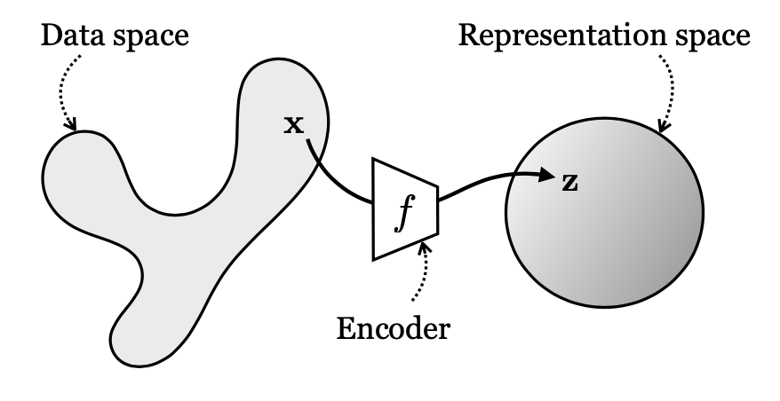
Some of the most salient learning methods within representation learning today include autoencoding, contrastive learning, clustering, and imputation; in this project, we focus on specifically on iterative approaches for the class of autoencoders.
Representation learning also has intricate ties to generative modeling, the subfield of deep learning that aims to generate new data by mapping a simple base distribution to complicated high-dimensional data, which is essentially the opposite goal of representation learning. Then, after learning an embedding space via representation learning, this embedding can then be sampled from to generate new data that mimics the original data, as demonstrated by variational autoencoders (VAEs), which we also explore in this paper.
Prior Literature
Relatively little literature exists regarding iteratively training dimensionality reduction or representation learning models. Vlahek and Mongus (2023) proposes an iterative approach for conducting representation learning more efficiently, specifically for the goal of learning the most salient features, which fundamentally diverges from our goal and also does not consider embedding robustness. Chen et al. (2019) introduces an iterative model for supervised extractive text summarization, though their objective of trying to optimize for a particular document by feeding a given document through the representation multiple times differs from ours. Cai, Wang, and Li (2021) finds an iterative framework for self-supervised speaker representation learning which performs 61% better than a speaker embedding model trained with contrastive loss, but mainly focuses on the self-supervision aspect of the model and optimizes purely for model test accuracy, not considering other metrics such as stability or robustness.
Overall, we find that the literature regarding iterative approaches to representation learning is already sparse; of the work that exists, most focuses on very specific use cases, and no work directly examines the robustness or stability of the model and embeddings themselves learned over time, rather optimizing purely for final model performance.
Iterated Representation Learning
Existing Dimensionality Reduction and Representation Models
Nowadays, there are a variety of approaches to effective dimensionality reduction. Below we cover three of the most common techniques.
Principal Component Analysis
Principal Component Analysis (PCA) has two primary objectives. First, maximizing sample variance of the newly transformed data, which is analogous to identifying and capturing the greatest (largest) directions of variability in the data (principal components or PCs). Formally, a PC is defined
\[v^* = \arg \max_v \frac{1}{N-1} \sum_{n=1}^N (x^T_n v - \bar{x}^T v)^2 = \arg \max_v v^T C v\]where \(C = \frac{X^T X}{n-1} \in \mathbb{R}^{d \times d}\) is the empirical covariance matrix.
The second objective is minimizing reconstruction loss, which is analogous to identifying the directions of variability to accurately and concisely represent data. Let \(U\) be the orthonormal basis projection matrix of eigenvectors of \(C\). Then we define reconstruction loss as
\[\mathcal{L}(U) = \frac{\sum_{n=1}^N ||x_n - U U^T x_n||^2}{N}\]Above, we observe that maximizing sample variance and minimizing reconstruction loss go hand-in-hand. Since PCA applies projections by multiplying vectors/matrices to the data, PCA is limited to the linear transformation setting, hence restricting its applicability in many modeling problems.
Autoencoders

Similar to PCA, autoencoders also aim to minimize reconstruction loss. However, autoencoders are not limited to just linear transformations, which enables autoencoders to learn more general lower-dimensional representations of data. Autoencoders are comprised of an encoder and decoder, where the encoder maps data to a lower-dimensional representation (embedding) via some function $f$, and the decoder maps the originally transformed data back to its original dimensional space via some function $g$.
End to end, the data space starts in \(\mathbb{R}^N\), is downsized to \(\mathbb{R}^M\) by \(f\), and then is reverted back to \(\mathbb{R}^N\) where \(N > M\). In this case, we can formalize the objective as follows:
\[f^*, g^* = \arg \min_{f,g} E_\mathbf{x} || \mathbf{x} - g(f(\mathbf{x}))||^2_2\]Variational Autoencoders
VAEs couple autoencoders with probability to get maximum likelihood generative models. Typically for encoding, VAEs regularizes the latent (hidden) distribution of data to “massage” the distribution into a unit Gaussian, and when reverting back to the original dimensional space, VAEs add noise to the output — hence, a mixture of Gaussians. By imposing a unit Gaussian structure on the learned embedding space, this allows VAEs to act as generative models by sampling from the Gaussian latent space to generate new data. Unlike traditional autoencoders, VAEs may have embedding spaces that are complicated (if not just as complicated as the data).
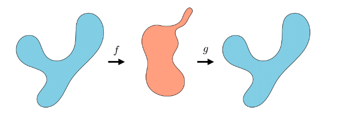
Formally, the VAE learning problem is defined by
\[\theta^* = \arg \max_{\theta} L(\{\mathbf{x}^{(i)}\}^N_{i=1}, \theta) = \arg \max_{\theta} \sum_{i=1}^N \log \int_{\mathbf{z}} \mathcal{N} (\mathbf{x}^{(i)}; g_{\theta}^{\mu}(\mathbf{z}), g_{\theta}^{\Sigma}(\mathbf{z})) \cdot \mathcal{N}(\mathbf{z}; \mathbf{0}, \mathbf{\mathrm{I}}) d\mathbf{z}\]Iterated Representation Learning
Proposed Framework
We now introduce the Iterated Representation Learning Framework (IRL) for autoencoders and VAEs. We start with IRL for autoencoders:
- Given design matrix \(X\), learn an autoencoder for \(X\).
- Using the decoder from above, reconstruct the data to get \(X'\) and compute its reconstruction loss.
- Using the reconstructed data \(X'\), repeat Steps 1 and 2 and iterate until the reconstruction loss converges or reaching iteration limit.
As for VAEs, we follow a similar procedure as above.
- Given design matrix \(X\), learn a VAE for \(X\).
- Using the decoder and adding Gaussian noise, reconstruct the data to get \(X'\). Compute its reconstruction loss.
- Using the reconstructed data \(X'\), repeat Steps 1 and 2 and iterate until the reconstruction loss converges or reaching iteration limit.
In this report, we examine how IRL is connected to representation, investigate several hypotheses about IRL, and conduct a preliminary case study of IRL on the MNIST dataset.
Preliminary Questions and Hypotheses
Motivated by how there may be unexplored stability properties of embeddings, our main hypotheses are twofold. First, iterated reconstruction loss per IRL can convergence with respect to the model. Second, learned embedding spaces can be reached via IRL, and that the number of iterations until convergence, loss at convergence, and such preserved features upon convergence could reveal meaningful properties of the true representation space, model, and data that are not immediately obvious from a standard autoencoder model.
More specifically, does the number of iterations until convergence have anything to do with how ``good’’ or stable the model or learned representation is? What does it mean if the reconstruction losses converge? What can we say about characteristics of the data that are maintained through iterations, and characteristics that evolve as the iterations go on? For example, if we observe that a model remains invariant to a certain feature, but becomes sensitive to new features of the data, what does this tell us about these particular features, our model, and the original data itself?
Perhaps most importantly, beyond the qualitative observations themselves, can we propose some sort of representation learning evaluation framework using iterated representation learning, e.g. rough guidelines on ideal number of iterations required until convergence, and what this says about how good a model is? Ultimately, we hope that using an iterated framework can serve as a general tool for (1) evaluating the stability or robustness of a representation learning model and (2) identifying the most core characteristics of a given dataset.
Case Study: MNIST Dataset
To evaluate IRL on a real-world dataset, we selected MNIST to test our hypotheses. We carefully designed our experiments, collected relevant data, and include our analysis below.
Experimental Design
For our experiments, we implemented IRL using the framework given above for the class MNIST digits dataset (due to its simplicity and intrepretability), where we preset the num_iterations. At every iteration, we initialize a new autoencoder model with Chadebec, Vincent, and Allassonnière’s (2022) pythae autoencoder/VAE library. The encoder architecture is formed by sequential convolutional layers from PyTorch.
We then trained the model, reconstructed the data, and saved the trained and validation loss. We also saved the original train/test and reconstructed train/test images of the first 25 datapoints to track how IRL progressed visually.
Autoencoder IRL Analysis
First, we take a look at the (log) mean squared error of our autoencoder over 30 iterations of IRL, given in the plot below.
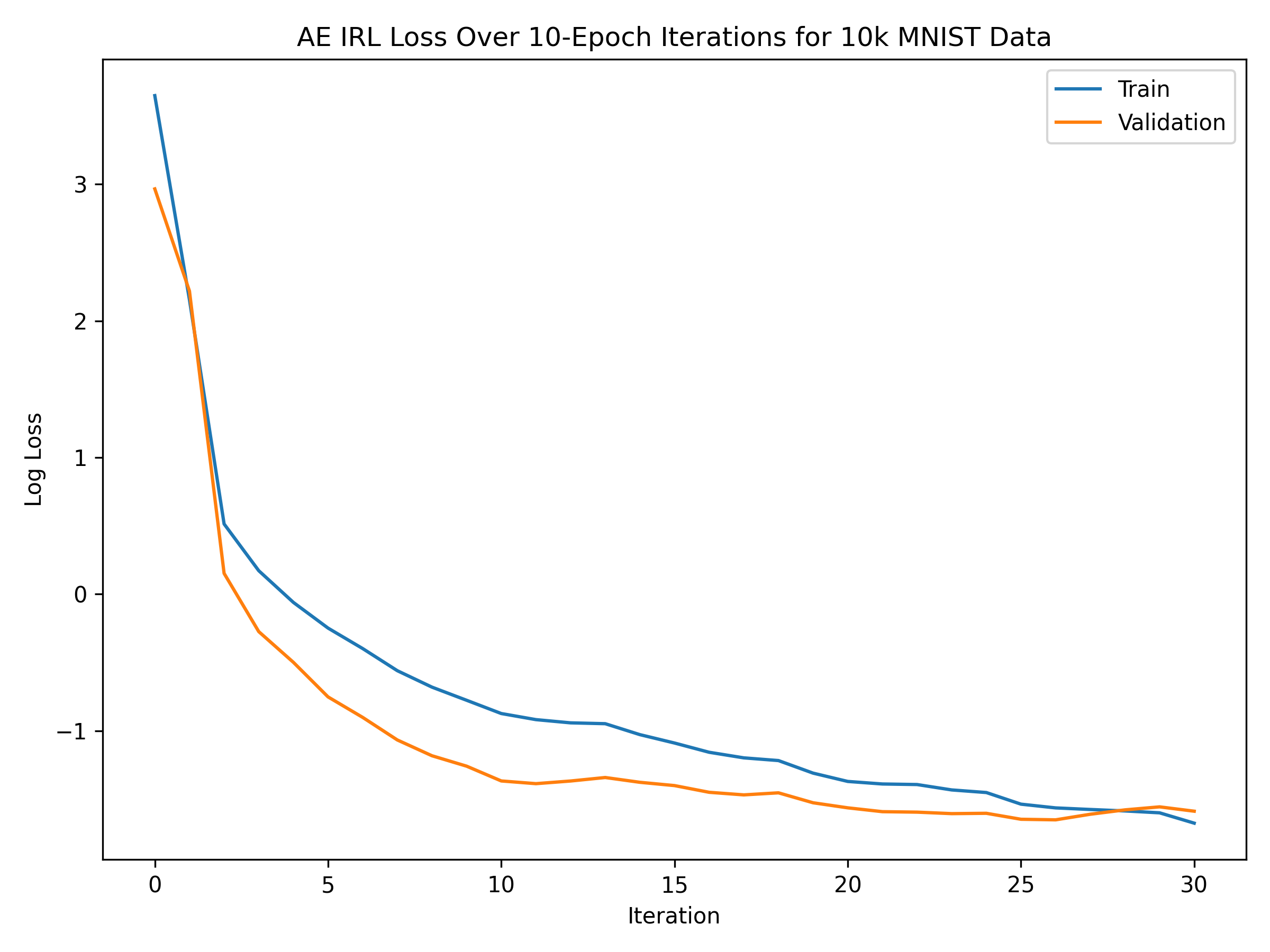
We notice that both the train and validation loss steeply decrease until around iteration 10, upon which the validation loss begins to roughly stabilize and converge. This confirms our intuition that the loss following an iterated approach should eventually converge, which we can theoretically verify by observing that if we ran \(n\) iterations, then as \(n\to\infty\), because the loss is lower-bounded by zero and should generally from iteration to iteration (since we are removing information from our data), we must eventually converge. We further hypothesize that the fact that the loss has converged means that the embeddings upon convergence have learned the most succinct, critical portion of the data.
We also notice that the number of iterations until convergence is very small; as mentioned, after about 10 iterations, it seems that the validation loss has roughly converged. We had hypothesized earlier that if the autoencoder converges after a small number of iterations, then that says something about the quality of the autoencoder architecture. Here, the fact that the loss converged after a small number iterations gives evidence for this hypothesis, since based on separate tests, this architecture indeed achieves relatively high classification accuracy for the MNIST dataset. We suggest that IRL can thus serve as a framework for evaluating the quality of an autoencoder on a particular dataset.
Additionally, the validation loss converges at a relatively small number (around 0.25 by iteration 10), meaning that the distance between the original and reconstructed data in a given iteration are very similar. Interestingly enough, the validation loss is actually consistently lower than the train loss, which suggests that the learned representations through this iterated approach actually generalize very well to unseen data, which is certainly a desirable quality of any model.
We also give the original and reconstructed data for iterations 1, 5, 10, 15, and 20, for both the train and test data, in the figures below.
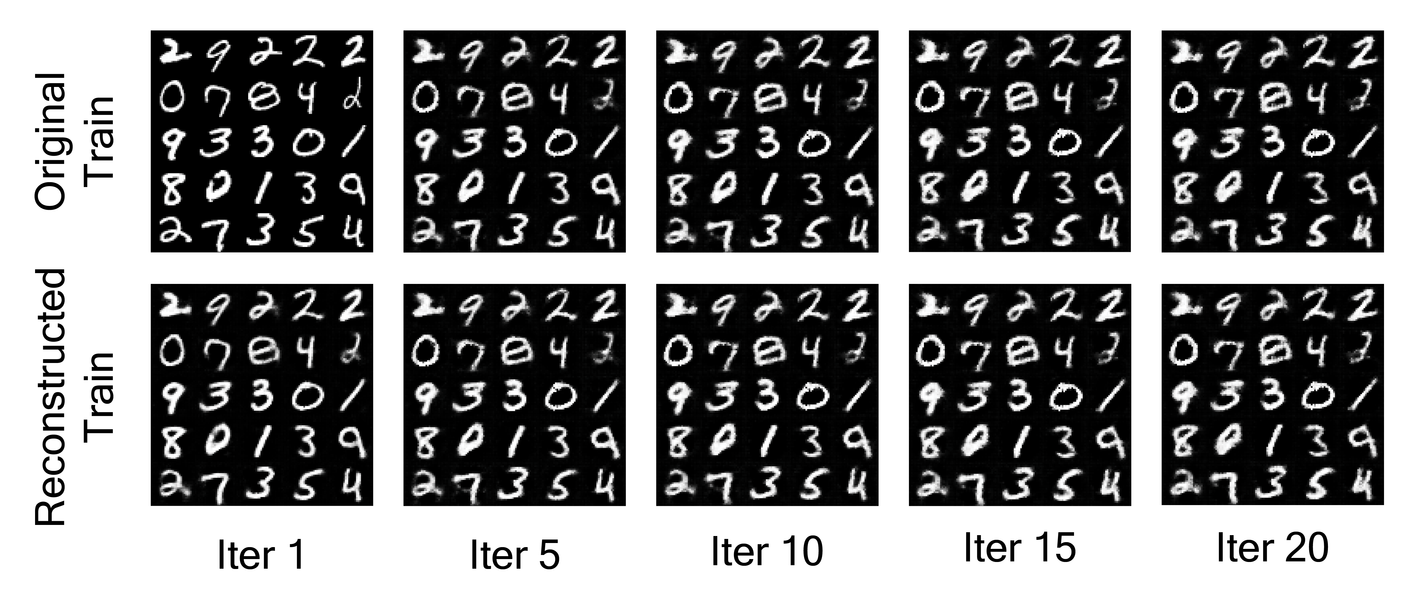
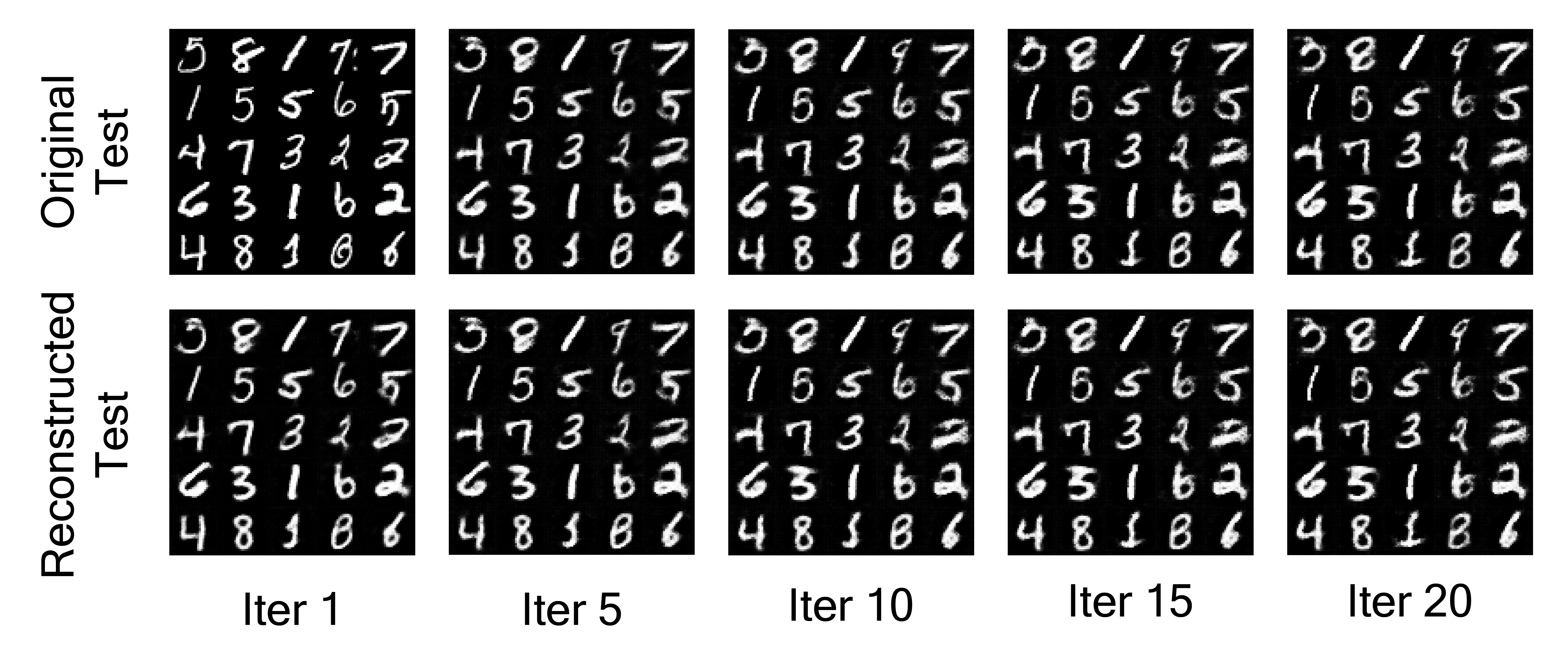
In the beginning, we see that the data starts losing resolution (e.g. the numbers become fuzzier and start losing their distinctness from the background), which makes sense because more iterations means more reconstructions that continue to accumulate reconstruction loss. The reconstructed images are also less clear than the originals due to the information that is lost from the encoding-decoding process.
Our key observation is that the reconstruction loss stabilizes around the 10th iteration, where the original test images and reconstructed test images look very similar — we hypothesize that this is the point where the autoencoder has learned to represent the data as succinct as possible while preserving the most critical information.
VAE IRL Analysis
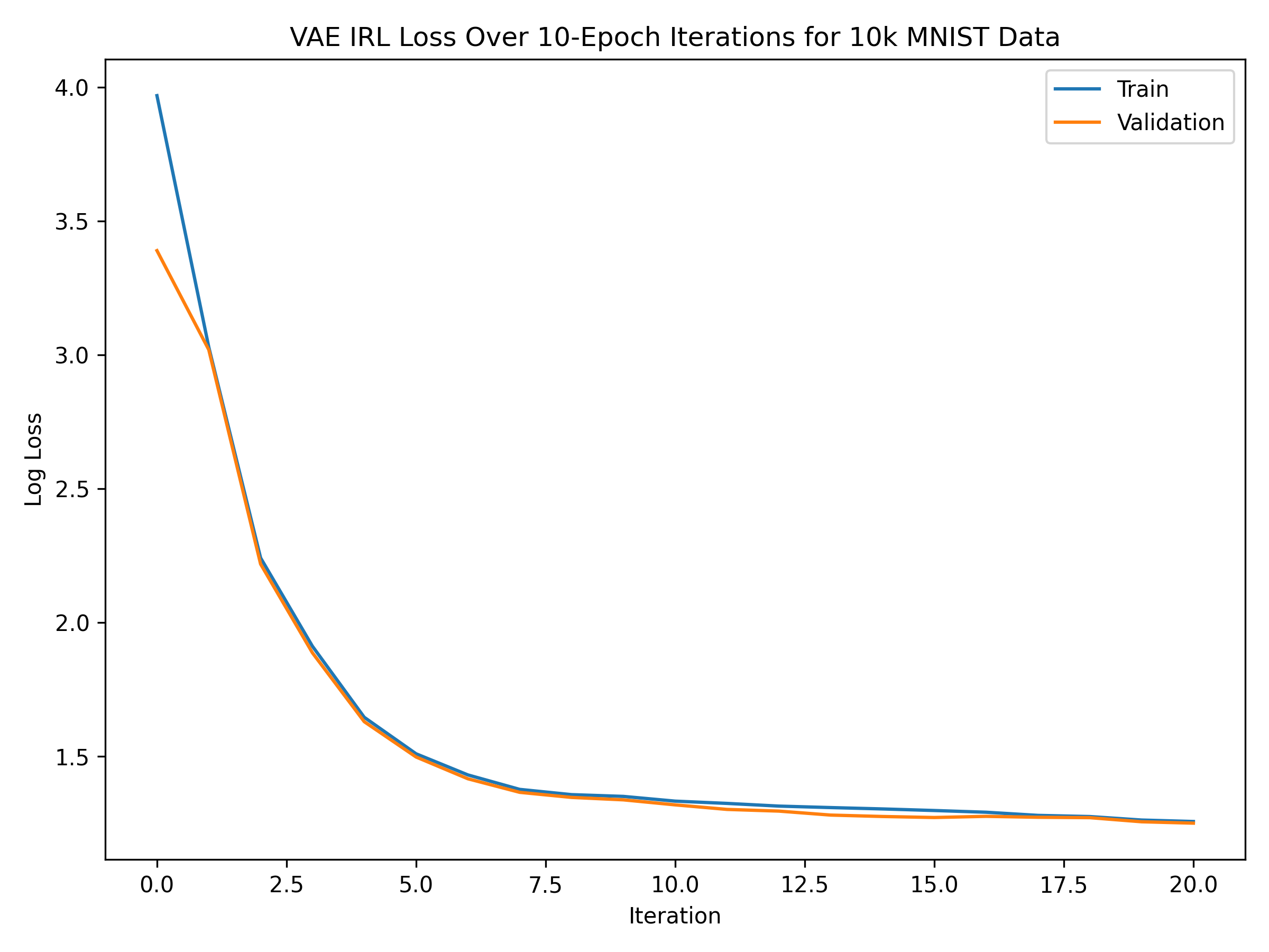
We similarly plot the log loss for our VAE, as well as the train, test, and sampled data over iterations in the figures below.
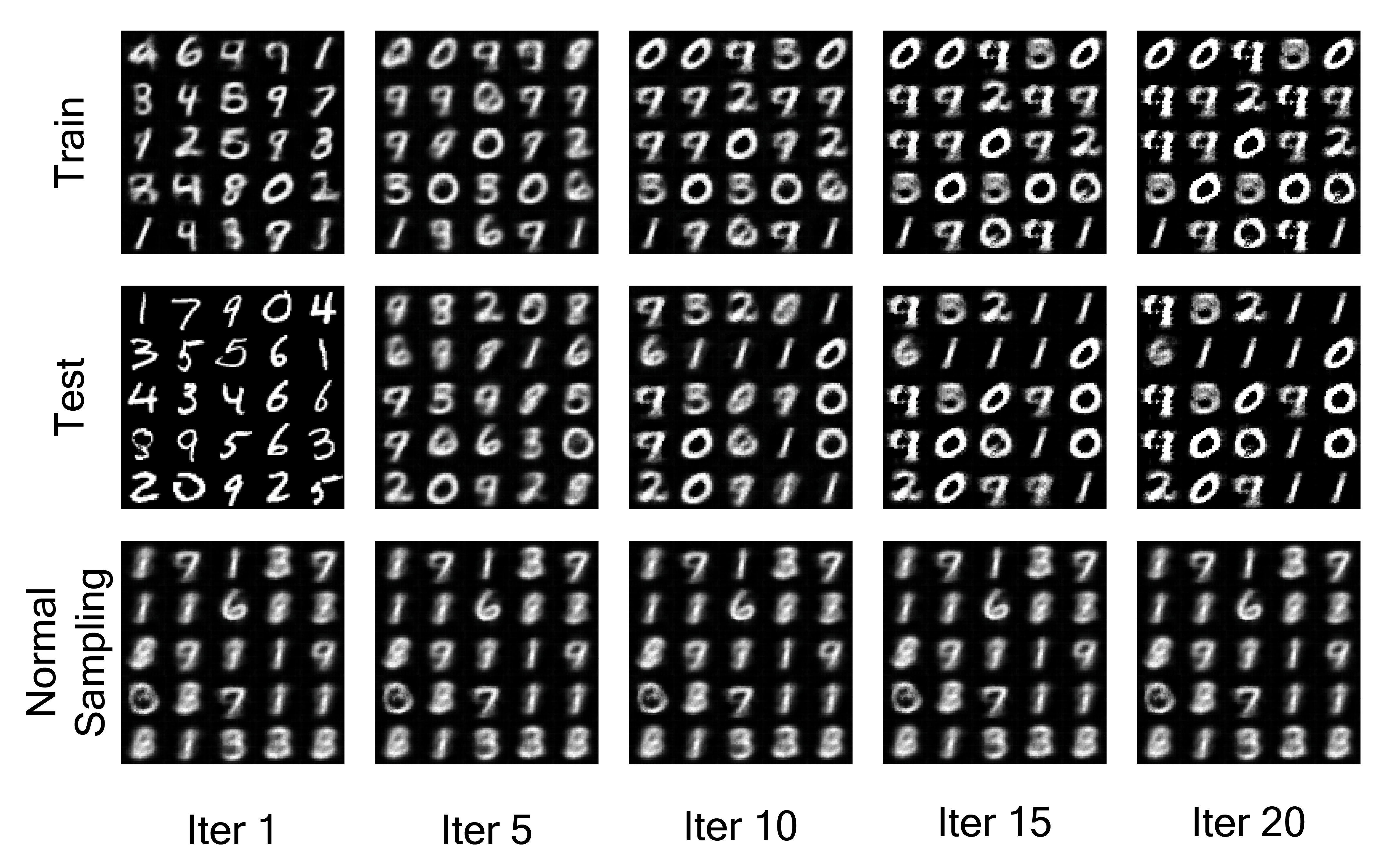
Unlike the autoencoder, the VAE’s train data becomes much more noisy across the 20 iterations. This is likely due to how the VAE injects noise in the reconstruction, which in this case resulted in the images to lose their distinctness. While the general shape is preserved (roundness, lines, etc), many of the numbers actually ended up merging together and losing their number shape altogether (e.g. some 6s, 3s, 9s all become 0s).
When comparing IRL on the autoencoder versus the VAE, we observe that the VAE’s log loss converges to a larger log loss than the autoencoder, which makes sense because the VAE’s decoding step adds noise to the images that therefore adds loss to the reconstruction. We also note that the both of the models experience steep drop offs in log loss initially, which means the first few iterations eliminated most of the noise in the data and preserved the features that we characterize as “stable”.
Discussion
Our proposed IRL framework considers how some features may be more important or more stable than others, and it aims to capture those features while eliminating the noise in the data. While traditional dimensionality reduction techniques have their merits, IRL takes those methods one step further by iteratively trimming away noise until convergence or termination. Throughout this project, we cover representation learning fundamentals and IRL can capitalize on the way they learn embeddings, and we also apply this framework to real world data on MNIST. We argue that in our case study of MNIST, IRL does converge in terms of both loss (log mean squared error converges) and reconstructions, which is a promising first step in the analysis of stability and fundamental characteristics of the data. Moreover, we showcase how the number of iterations until convergence has significance, serving as a benchmark for how good an autoencoder/VAE is on a given dataset. Although VAE’s reconstructed images were more noisy, that’s by nature of the VAE, and we still observe that the fundamental features of the data (lines vs circles) are still preserved throughout iterations.
There are a variety of directions we’d like to continue to explore with this project, given more time.
- We were only able to run a limited number of experiments due to computational power and the duration of time to train a full IRL from start to finish for, say, 30 iterations. Given more time, there are multiple other experiments we’d like to run, including training on other datasets and trying out the performance on different autoencoder architectures to better understand the properties of this iterated approach. Another thing we’d like to evaluate the empirical performance of, but also couldn’t due to computational constraints, is how a single autoencoder with 20 times as many neurons as some basic autoencoder compares to the basic autoencoder trained using IRL for 20 iterations.
- We’re also curious to further explore the theoretical guarantees provided by IRL, including rigorous bounds on convergence. We’re also very interested in exploring whether any of our observations from IRL can generalize to other classes of deep learning models.
- We’d lastly look into ways to make IRL more computationally tractable. As mentioned, our experimentation was heavily limited due to the computational cost of training a new autoencoder during every iteration. If possible, we’d like to look for optimizations of this framework that still preserve the desired methodology.
Overall, Iterated Representation Learning serves as a framework to evaluate stability-related properties of data, which we believe to be an important but overlooked standard for representation learning. Our case study of MNIST shows promise for empirical convergence guarantees on certain datasets, and we hope that our work lays the foundation for future representation discussions with respect to stability.