Investigating Vision Transformer-Based Models for Closure Modeling of Fluid Dynamical Systems

Project Report for 6.s898 Deep Learning (Fall 2023)

Motivation and Background

Over the past decade, deep learning models have increasingly been used for modeling time series data for fluid dynamical systems. One of the most recent applications is in forecasting weather with deep learning models being developed by tech giants including NVIDIA and Google with reasonable prediction accuracy compared to conventional numerical weather prediction. While these models completely replace traditional numerical weather models with deep neural networks (i.e., “surrogate modeling”), in general, deep neural models can also be used to augment existing numerical solvers and methods .

Training deep neural models to completely replace numerical solvers requires a lot of data, which might not be available due to constraints with sensor and satellite usage associated with collecting ocean and weather data. Additionally, these surrogate models are completely data-driven and could lead to non-physical predictions (lack of volume preservation, and non-conservation of physical laws) if these needs are not explicitly attended to during training . A huge advantage of these models is their very low computational cost during inference compared to using numerical solvers . Another approach is to use closure models that augment low fidelity (low resolution) numerical simulations with a neural network (i.e., a closure term) to predict high fidelity (high resolution) forecasts . This approach could lead to some conservation of physical laws since it builds upon conventional numerical solvers that obey physical equations like PDEs, with a lower computational cost compared to directly running high-fidelity numerical simulations.

In closure modeling, we are interested in solving the following problem: Here, we describe the case of closure modeling with loss of accuracy due to low numerical resolution which leads to loss of sub-grid scale processes, and sometimes even truncation and discretization errors. But there could also be closure due to missing or unknown physics, incorrect parameters, etc. .

Consider a low-fidelity model (low resolution):

$$ \frac{du_{LF}(t)}{dt} = f(u_{LF}(t)) \tag{1} $$

and the high fidelity (high resolution) equivalent model:

$$ \frac{du_{HF}(t)}{dt} = f(u_{HF}(t)) \tag{2} $$

The purpose of the closure in this context is to augment the low fidelity model with a neural closure model $NN(u_{LF}(t))$, such that:

$$ u_{HF}(t+1) = \int_{t}^{t+1} \bigg(\frac{d u_{LF}}{dt} + NN(u_{LF}(t)) \bigg) dt \tag{3} $$

Previous works for neural closure models have used neural ODEs and neural DDEs . However, these methods require coding an adjoint equation, which could be difficult for complex 2D problems. Another approach has been to use local CNNs for turbulent models . More recently, vision transformers have been shown to be very successful for image recognition , and have also been adapted to predict the mapping between two infinite-dimensional function spaces using Neural Operators (more details in the following sections). These adaptive neural operators have also been used for predicting fluid flows like flow past a cylinder using experimental data for training . However, to the best of our knowledge, the usage of vision transformers for closure modeling of 2D fluid flow fields has not been explored.

Another issue with using neural networks for solving fluid dynamics PDEs is unstable recursive predictions, due to the exponential growth of accumulated errors across time. Some papers have explored ways to limit this exponential error growth by using custom loss functions , and adding additional spectral networks to limit error growth . In this project, we attempt to achieve stable long roll-outs by first training models for one-time-step predictions and then fine-tuning for long roll-out, inspired by .

Methods and Experiments

Test case setup

In this project, we develop and investigate methods to augment low-fidelity (low-resolution) numerical simulations of flow past a cylinder with deep neural networks and compare them with high-fidelity (high-resolution) numerical simulations. The neural closure aims to learn the missing subgrid-scale processes and truncation and discretization errors in the low-fidelity simulation and augment it to match the high-fidelity simulation

Data generation

We use data generated from numerical simulations for two-dimensional flow past a cylinder . We employ the MIT-MSEAS 2.29 Finite Volume framework to solve the Navier Stokes equations at different numerical resolutions and fidelities. Figure Figure 1 shows the geometry, inlet conditions, and boundary conditions used for the numerical simulations. The test set-up consists of a rectangular geometry of length 15m and height 5m. A cylinder is placed 2m upstream with a diameter of 1m. The inlet velocity is set to 2m/s horizontal velocity and no vertical velocity. The boundary conditions are set to outflow conditions on the right boundary and free slip on the top and bottom boundaries. We use Reynolds’s number of $Re=200$. The Reynolds’s number is a key parameter that affects the regime of solutions observed, at $Re\geq 200$, complex periodic patterns can be observed known as wakes, eddy shedding, or Karma vortex streets . It is in this complex regime that we are interested in applying our deep learning methods.

Figure 1: Schematic of the flow past a cylinder setup used to generate data

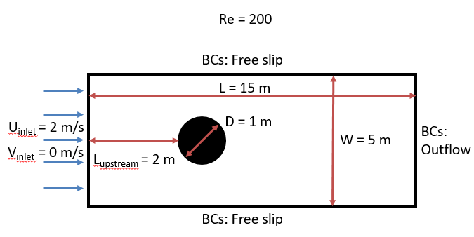
To generate the high-fidelity (high-resolution) data we use a resolution of 200x600. For the low-fidelity (low-resolution) data, we use a resolution of 50x150. The MIT-MSEAS 2.29 numerical simulation uses second-order finite volumes and a time-step of 0.000625s. The diffusion operator was discretized using central boundary fluxes. For advection, we use a total variation diminishing (TVD) scheme with a monotonized central (MC) symmetric flux limiter. For numerical time integration, we use a rotational incremental pressure correction scheme. The reader is directed to for more details on the numerical schemes. We simulated the flow for a total of 30s, and the data is saved once every 0.03125s, for a total of 9600 snapshots. We observed fully developed eddies after 15s. An eddy sheds approximately every 2s, so we find a shedding period of about 4s.

Data usage for deep learning

We save the u and v velocity fields, as well as the time derivatives (which act as the numerical approximation of the RHS terms (dynamics terms) of the PDEs being solved).

Thus we save a tensor of size $9600 \times 4 \times \text{num. horizontal cells} \times \text{num. vertical cells} $, for each numerical resolution, where 9600 is the total number of time steps saved, and 4 indicates 4 channels for the 2 velocities and 2 time derivatives (horizontal: u and vertical: v). To maintain the same grid size for deep learning, we down-sample the high-fidelity data using linear interpolation to have the same size as the low-fidelity data.

For deep learning, we neglect the first 4800 snapshots as spin-ups to reach a fully developed flow state. Then we use the next 3600 snapshots for training, 600 snapshots for validation, and 600 snapshots for testing.

We created a custom data class with a data loader to feed randomized sequences of required sequence lengths from the training set for training. For inference, we feed the snapshots one by one from the test data set.

Deep learning model

For this project, we initially tried to explore architectures inspired by Fourier neural operators . These operators learn the relationship between two infinite dimensional spaces, by using kernels in the Fourier space instead of physical space. Since multiplications in Fourier space are akin to convolutions in physical space, these models can learn powerful infinite dimensional mapping at reduced computational cost. In particular, we were interested in Adaptive Fourier Neural Operators , which build upon vision transformers. Like vision transformers, these models first split the input image into patches and tokens with positional embedding. However, instead of relying on QKV (Query, Key, Value) attention mechanisms, they perform a 2D spatial Fourier transform of the tokenized representation and use MLPs (which act as convolution, since multiplication in Fourier space is convolution in physical space) to learn the mapping between input and output images. Since these models don’t involve self-attention, they have significantly fewer parameters compared to vision transformers and can even outperform them in certain tasks. Figure Figure 2 shows a schematic comparing a regular vision transformer with AFNO. However, we were not able to further explore this architecture due to time constraints.

Figure 2: Schematic of the difference between a regular QKV attention based vision transformer and an AFNO layer

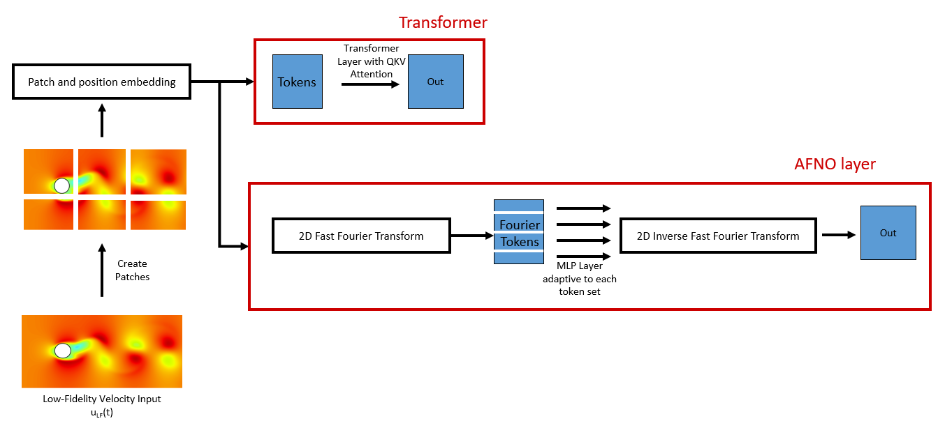
Instead, we focus on utilizing vision transformer-based architectures for our closure modeling task. Although they have a higher number of parameters than AFNO, vision transformers rely on self-attention that can learn long-range physical dependencies, and are hence well suited to our task.

Single time-step predictions

We first focus on a framework that just predicts output for the next time step, i.e., single time-step predictions. This is a simpler task than recursive or long roll-out predictions which we will discuss in the following sections.

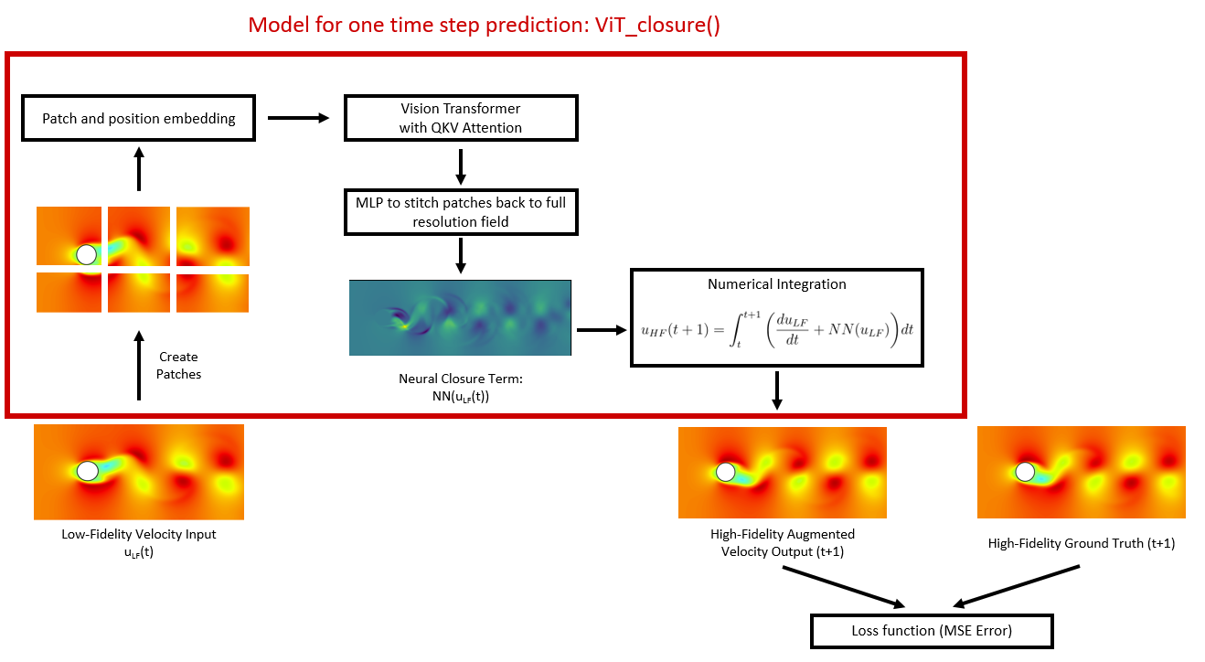
Figure 3 contains a flowchart of how our Vision Transformer-based closure model “ViTClosure()” works. In the first part of the architecture, a vision transformer-based architecture takes in a low fidelity velocity field at time t as input and returns the closure term (which is similar to a time derivative field) at time t+1.

First, a 2D CNN transforms the input low fidelity 2D velocity field at time $t$ into patches
Next, a layer adds positional embedding and creates tokens. In this project, we use learned absolute positional embeddings.
Next, the tokens are passed through a vision transformer with many attention layers with multi-headed attention heads.
Next, we have a layer that applies layer norm to the final output of the vision transformer. Here the output would be of size $\text{Batch size} \times \text{Num. of tokens} \times \text{Hidden dimension}$. Since we need an output field of the same dimension as the input field, we use an MLP for this transformation. We call this output closure term $NN(u_{LF}(t))$.
Next comes a numerical integration step which combines the low fidelity numerical solver (which provides $\frac{d u_{LF}}{dt}$) with the neural closure term $NN(u_{LF}(t))$, to predict the high-fidelity field $u_{HF}(t+1)$, shown in Eq. (4).

$$ u_{HF}(t+1) = \int_{t}^{t+1} \bigg(\frac{d u_{LF}}{dt} + NN(u_{LF}(t)) \bigg) dt \tag{4} $$

Figure 3: Flow chart of the model used for closure modeling with single time step predictions. Please see text description for more details

Loss functions

Finally, we compare the predicted high-fidelity field $u_{HF}(t+1)$ and neural closure term $NN(u_{LF}(t))$ with the ground truth simulations. Similar loss functions have been used in neural closure models based on neural-ODEs . In this work, we use a weighting factor that is a hyperparameter that can be tuned to weigh either the state errors or closure term errors depending on the application. The loss function is defined in Eq. (5).

$$ \mathcal{L}_{\text{weighted}}(.;\lambda) = \text{MSE}\bigg(u_{HF}(t+1),u_{HF_{true}}(t+1)\bigg) + \lambda \text{MSE}\bigg(NN(u_{LF}(t)),\text{True closure}(u_{LF}(t))\bigg) \tag{5} $$

Then, we use backpropagation with the Adam optimizer and a cosine learning rate to optimize the model parameters.

Fine tuning for recursive predictions

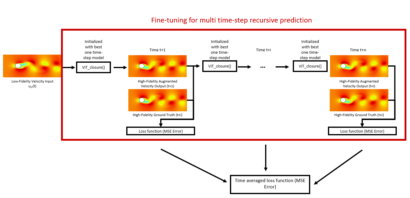
Now that we have a model trained for single time-step predictions, we move on to multiple time-step predictions or long roll-out predictions. Achieving long roll-out predictions is hard due to the exponential accumulation of errors during recursive predictions. Hence a small error at timestep t+1 could lead to huge errors after a few more timesteps. have recently worked on achieving stable long roll-outs using spectral data augmentations. In this project, we try a different approach by using fine-tuning, and using a loss function inspired by . The flowchart of the fine-tuning process is shown in Figure 3. The description is as follows:

We first initialize the model using the best-performing model of the single-time step prediction, i.e., the best ViT-closure() model.
Next, we recursively use the ViT-closure() model, and feed the output at time t+i as input to the model at time t+i+1.
Finally, we average all the losses across time Eq. (6). and backpropagate through time.

$$ \mathcal{L}_{\text{recursive}}=\frac{1}{n}\sum_{t=1}^n \mathcal{L}_{\text{weighted}}(.;t,\lambda) \tag{6} $$

where ‘n’ is a hyperparameter that determines how many times the model is propagated recursively during fine-tuning.

Figure 4: Flow chart of the fine-tuning step used to train the closure model to predict recursively for long roll-outs. Please see the text description for more details

Results and Analysis

We ran many experiments for the flow past a cylinder set-up with high-fidelity (high-resolution) data of resolution 200x600 and low-fidelity (low-resolution) data of resolution 50x150. The high-fidelity run was downsampled as described previously to achieve the same grid size as the low-fidelity data for comparison. We used one NVIDIA RTX A6000 GPU for all the training and inference runs.

Single time-step predictions

First, we train the single time-step prediction model using the procedure described previously. We tried many runs (~ 20) by varying the key hyperparameters such as the global batch size between 1 and 16, the embedding dimension between 64 and 256, the number of attention layers between 3 and 9, the number of attention heads between 5 and 10, the patch size between 5 and 10, and the weightage in the loss function $\lambda$ between 0 and 1.

Increasing the batch size led to faster training, but higher GPU memory requirements. With a batch size of 1, it took around 8 minutes of wall-clock time for one epoch of training. We observed the best training results with a loss function weightage $\lambda$ of close to 0, this may be because we ran the numerical solver offline to obtain the low-fidelity derivatives and ground truth closure, which is not as accurate as obtaining these values online during training. The other hyperparameters decreased training errors but the validation error after 50 epochs of training was around 0.03 m/s compared to the average velocity field of 2 m/s (so about 1.5\% relative error). Regularization and avoiding overfitting of the model needs to be investigated further in future work.

For the GIFs below, we use the best-trained model, which was trained using a batch size of 16, embedding dimension of 128, number of attention layers of 6, number of attention heads of 10, patch size of 5, and weightage in the loss function $\lambda$ of 0.05.

Using this model, we can visualize the attention layers, to identify which features have been most useful for closure modeling. Figure 5 shows the attention map of multiple patches on the low-fidelity u velocity input at the same time step. We can observe that the most important feature seems to be the phase (whether the eddy is facing upward or downward) of the eddy shed right at the cylinder, and the other eddies downstream. We can also see that there is very little attention near the inlet and top and bottom boundaries since those values are set as inputs to the simulation.

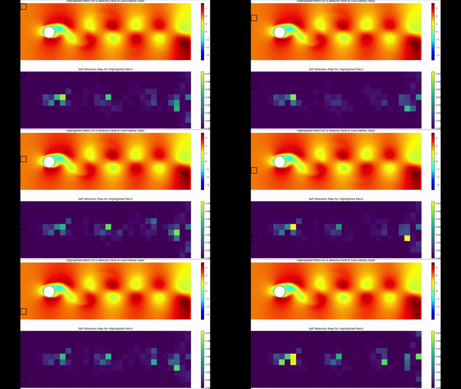
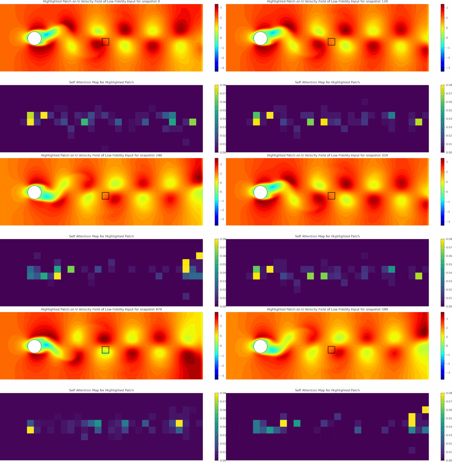
Figure 5: GIF shows the attention map of multiple patches on the low-fidelity u velocity input at the same time step

Figure 6 shows the attention map of a single patch on the low-fidelity u velocity input at different time steps. We can again observe that the attention map follows the eddy shedding at all times. These two plots indicate that the model can identify that the eddies are the most important features, and the inlet and boundaries are not that critical for predicting the flow field. However, this may not be true if we are attempting to do closure modeling between simulations with different inlet and boundary conditions, which can be further investigated in future work.

Figure 6: GIF shows the attention map of a single patch on the low-fidelity u velocity input at different time steps

Now that we know that our model focuses on the most important features for closure modeling, we can compare the field plots of the high-fidelity predictions using the model.

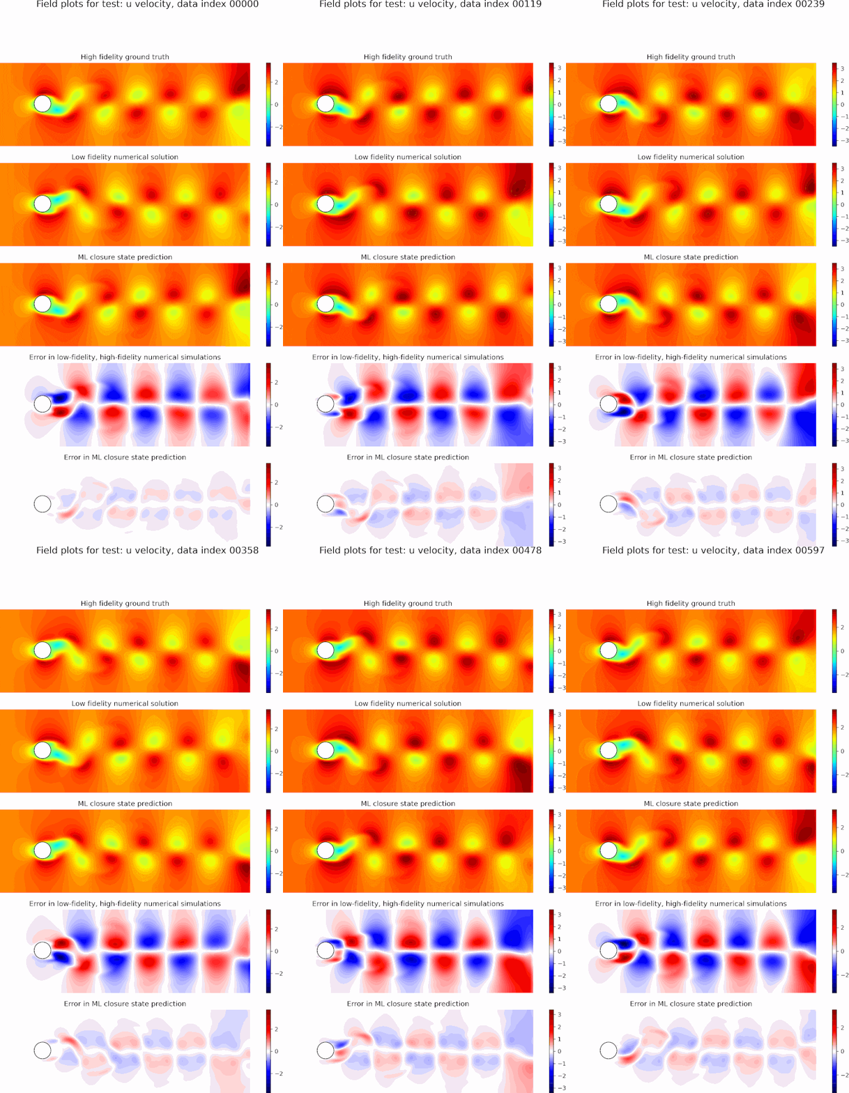
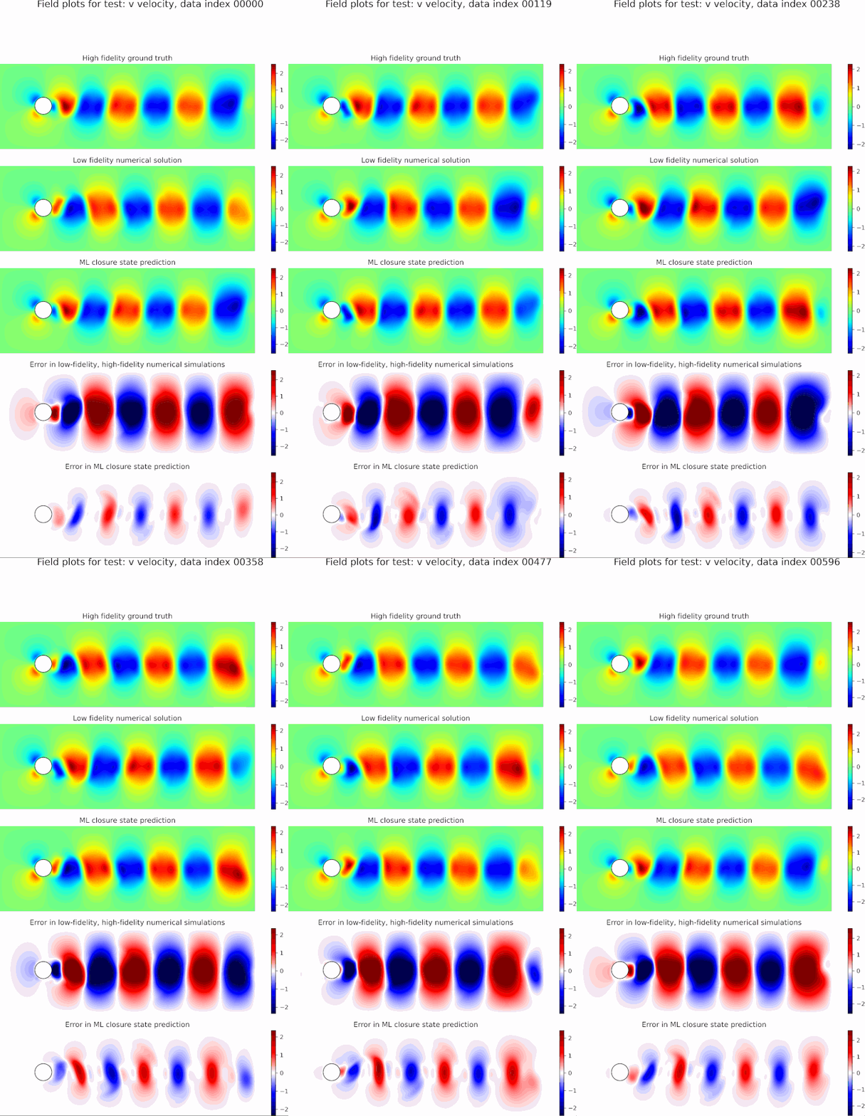
Figure 7 and Figure 8 show the comparison of the neural closure model predictions, and predictions with just low-resolution simulations. We can observe that the neural closure model prediction (3rd row) performs way better than the low-fidelity simulations (2nd row). The low-fidelity simulation is out of phase compared to the high-resolution ground truth, but our neural closure model is able to augment the low-fidelity simulation and learn the true phase and missing sub-grid scale processes!

Figure 7: GIF shows comparison of low fidelity prediction and augmented neural closure single step predictions for u velocity for testing times

Figure 8: GIF shows comparison of low fidelity prediction and augmented neural closure single step predictions for v velocity for testing times

Fine tuning for recursive predictions

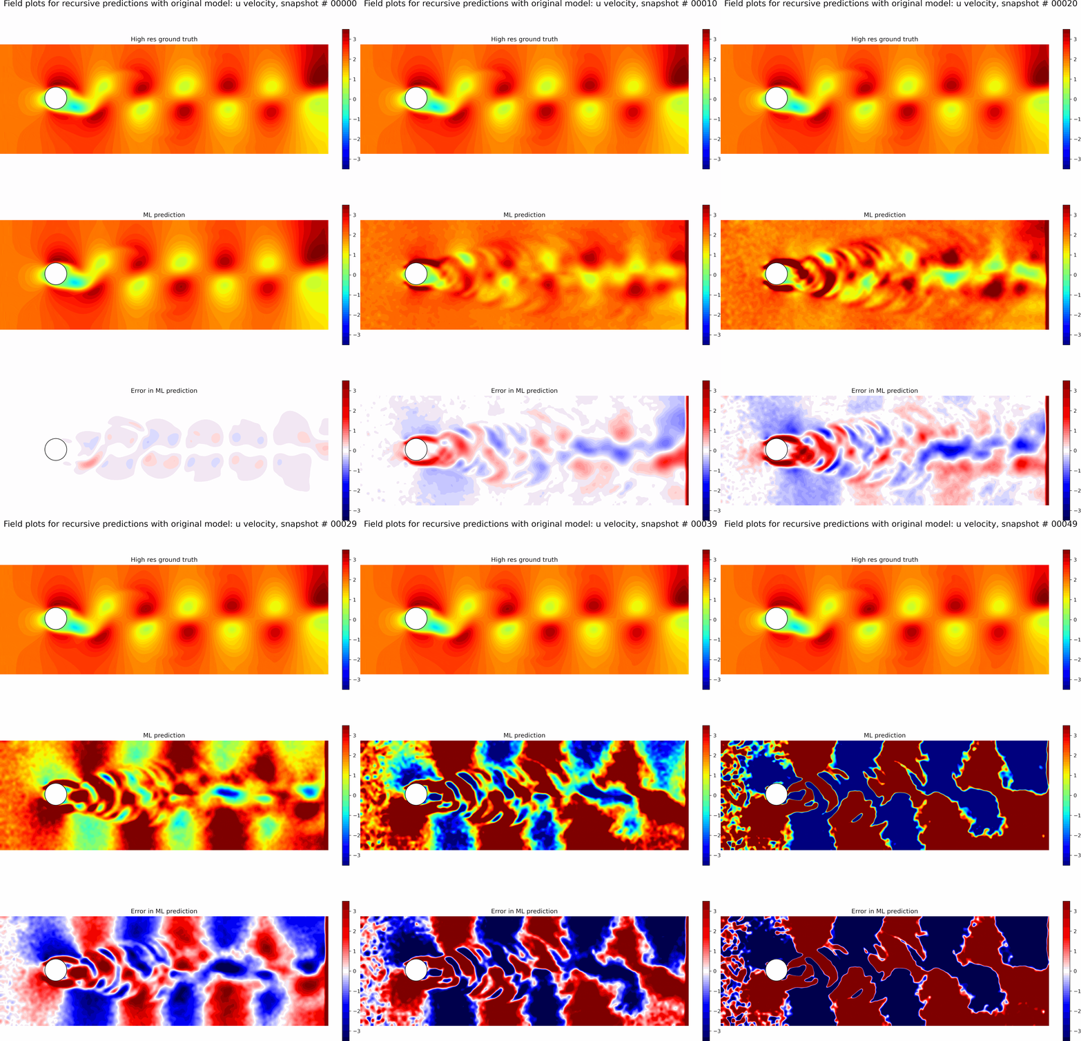
Next, we evaluate the capabilities of the best model from the single time-step predictions for recursive predictions. We set the initial conditions to be the first snapshot in the testing data set and perform recursive predictions as described before for 50 time steps. The resulting predictions and error fields are shown in the GIF in Figure 9. We can see that the errors grow exponentially even before a few recursive predictions, and the model is incapable of any accurate long-term predictions. The predictions quickly become out of phase compared to the ground truth.

Figure 9: GIF shows the result of recursive predictions by the best single time-step prediction model

Next, we initialize a new model using the weights from the best single time-step predictions and perform fine-tuning as described previously.

We explore multiple values of $n$, which is a hyperparameter that controls how long the recursive sequence lengths used for fine-tuning are. We found the ideal value of ‘n’ to be $5$ timesteps. Using $n<5$ led to inaccurate recursive predictions, using $n>5$ did not lead to much improvement in accuracy but increased training costs due to requirements to backpropagate through long-time sequences.

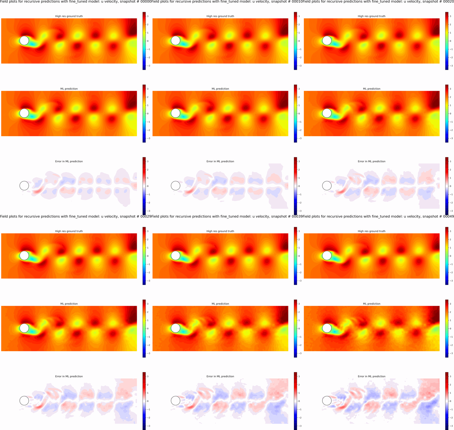
The resulting predictions and error fields after fine-tuning are shown in the GIF in Figure 10. We can observe that the model predictions remain in phase with the ground truth, and the error fields are low up to 50 timesteps. We can see that even though we only fine-tuned with sequence lengths of 5, the resulting model is stable for long roll-outs of up to 50-time steps. However, this could be because eddy shedding in flow past a cylinder is somewhat periodic, which aids in some generalization.

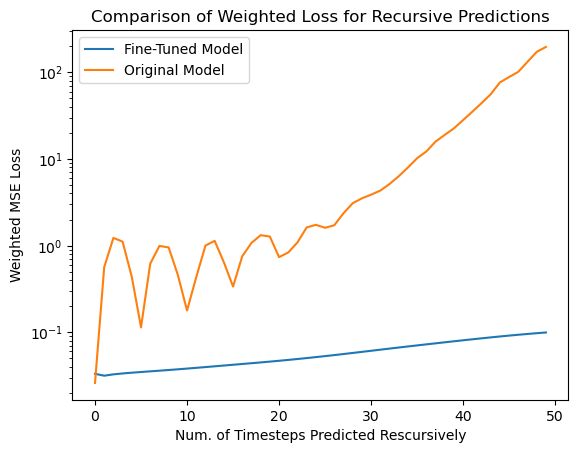
Figure 10: GIF shows the result of recursive predictions after fine-tuning

Finally, to show the effectiveness of fine-tuning, we compare the weighted loss of the original best single-time step model and the resulting best-fine-tuned model for long roll-out predictions of 50-time steps in Figure 11. We can see that the original model sees exponential growth of errors up to 2 orders of magnitude higher in just 10 recursions while the fine-tuned model is stable up to 50 recursions. Thus, we can see that our fine tuning mechanism allows for stable roll outs well beyond the training sequence length.

Figure 11: Comparison of the weighted loss of the original best single-time step model and the resulting best-fine-tuned model for long roll-out predictions of 50-time steps

Conclusions and Future Work

In this project, our key contributions have been

Extending vision transformer-based models for neural closure modeling for an idealized 2D flow field (eddy shedding from flow past a cylinder). We observed a reduction in error fields by up to 95\% using neural closure augmentations, compared to just using the low-fidelity output.
Developing a fine-tuning procedure to achieve long recursive predictions, i.e., we have achieved stable long roll-outs for ~50 timesteps by training on just ~5-time step sequences.

Some of the limitations of our model and future work are:

Scalability and usage of large amounts of VRAM for training: Training with a batch size of 1 takes up 7 GB of VRAM for the 50x150 field. Training with parallel GPUs or other more efficient transformer token mixing models like Adaptive Fourier Neural Operators (AFNOs) needs to be explored to increase the batch size or number of grid points.
Numerical integrator inside closure model: We use a forward Euler numerical solver for the numerical integrator during closure modeling, however more stable and accurate solvers like DOPRI5 or RK4 need to be investigated.
Offline training: Right now, our model uses offline data generated by a numerical solver. For complete accuracy, we would need to integrate the numerical solver (written in MATLAB or FORTRAN) into the training code and allow it to compute the low-fidelity derivatives online during training.
Effect of periodicity: The eddy shedding in the flow past a cylinder is somewhat periodic which may aid the deep learning model during training. The model needs to be tested on more realistic flows like gyre flow, or real ocean velocity fields, to test its true capabilities.