Semi-Supervised Domain Adaptation using Diffusion Models
6.S898 Project
Abstract
Recently, there has been a breakthrough in image manipulation using Contrastive Language-Image Pretraining (CLIP). Recent work shows that GANs combined with CLIP can translate the images to unseen domains
Introduction & Background
Diffusion models
Diffusion Denoising Probabilistic Models (DDPMs) were introduced by Ho et al. as a novel approach in the field of generative models
The diffusion process is a Markov chain that adds Gaussian noise to the data over a series of steps. This process can be described mathematically as:
\[x_{t} = \sqrt{\alpha_{t}} x_{0} + \sqrt{1 - \alpha_{t}} \epsilon\]where $x_{t}$ is the data at step $t$, $x_{0}$ is the original data, $\alpha_{t}$ is a variance schedule, and $\epsilon$ is Gaussian noise.
The reverse process aims to denoise the data, starting from the noisy version and progressively removing noise. It’s modeled as:
\[x_{t-1} = \frac{1}{\sqrt{\alpha_{t}}}\left(x_{t} - \frac{1-\alpha_{t}}{\sqrt{1-\alpha_{t}}} \epsilon_{\theta}(x_{t}, t)\right)\]with $\epsilon_{\theta}(x_{t}, t)$ being a neural network predicting the noise. This neural network usually has a UNet architecture with downsampling layers, upsampling layers, and a bottleneck.
The training objective is to minimize the difference between the predicted noise $\epsilon_{\theta}(x_{t}, t)$ and the actual noise $\epsilon$. This is done using a variant of the mean squared error (MSE) loss:
\[\min_\theta \mathbb{E}_{x_0 \sim q(x_0), w \sim \mathcal{N}(0, I), t} \left\| w - \epsilon_{\theta}(x_t, t) \right\|^2_2.\]DDIM (Denoising Diffusion Implicit Models) paper
where, $z \sim \mathcal{N}(0, I)$ and $f_\theta(x_t, t)$ is a the prediction of $x_0$ at $t$ given $x_t$ and $\epsilon_\theta(x_t, t)$:
\[f_\theta(x_t, t) := \frac{x_t - \sqrt{1 - \alpha_t}\epsilon_\theta(x_t, t)}{\sqrt{\alpha_t}}.\]DDIM process allows for the use of different samplers by setting $\sigma_t$ to different values. In particular, setting $\sigma_t = 1$ makes the process a Markov process equivalent to DDPM while setting $\sigma_t = 0$ makes the process deterministic and allows for almost perfect inversion. DiffusionCLIP method leverages the deterministic nature of the process for image manipulation.
Image manipulation with CLIP
CLIP is a model for joint image-language representations which is trained on a large dataset of image-text pairs
where $ \Delta T = E_T(y_{\text{tar}}) - E_T(y_{\text{ref}}), \Delta I = E_I(x_{\text{gen}}) - E_I(x_{\text{ref}}). $
$E_I$ and $E_T$ are CLIP’s image and text encoders, $y_{\text{ref}}, x_{\text{ref}}$ are the source domain text and image, and \(y_{\text{tar}}\) is a text description of a target and \(x_{\text{gen}}\) denotes the generated image.
Related Work
Recent work in the field discovered an alternative way of manipulating image attributes using pre-trained diffusion models
Although this method is still in development (as it was our initial idea for domain adaptation which did not succeed), the latent space suggested by the authors can be used for a more powerful idea which is unsupervised domain adaptation. By smoothing the test images at appropriate noise level, one can classify whether the image possesses a given attribute. Then one can make training and test distributions close to each other by manipulating the attributes of interest. This direction is of our future interest to explore.
Another area of current research is trying to use GANs (also guided by the CLIP loss) for image manipulation
An alternative method for manipulating and editing images is mixing latents of source and target
Another method for image editing is classifier guidance which adds classifier gradients in the reverse process to control the generation process
Our Contribution
We demonstrate capabilities of text-guided diffusion to perform domain adaptation in a semi-supervised setting (e.g., unseen attributes of the target domain). To the best of our knowledge, this is the first work that shows the power of diffusion models in performing domain adaptation when the difference between the train and target domains can be described in a short prompt.
Methodology
A frequently encountered problem in supervised learning is one where we have training data from one domain (the source domain) but we want to conduct inference on data that comes from a different but related domain (the target domain) that can be described using text. Specifically, we want to focus on the setting where we have access to an adequate number (for training) of observations from the source domain (a subset of which are labelled) and we want to conduct inference (eg. classification) on unlabelled observations from the target domain. An additional constraint is that we only have a limited number of observations from the target domain so it is infeasible to learn the target distribution. Here, we deal with image data.
DiffusionCLIP
We first train a diffusion model on both labelled and unlablled images from the source domain. This diffusion model is first used to convert input images (from source domain) to the latent. Then, the reverse path is fine-tuned to generate images driven by the target text (text decription of target domain), guided by the CLIP loss. The details are given in the subsequent sections.
DiffusionCLIP Fine-tuning
In terms of fine-tuning, the DiffusionCLIP model
Loss Function
The objective function is given by:
\[\mathcal{L}_{\text{direction}} (\hat{x}_0(\theta), y_{\text{tar}}; x_0, y_{\text{ref}}) + \mathcal{L}_{\text{id}} (\hat{x}_0(\theta), x_0)\]where $x_0$ is the original image and \(\hat{x}_0(\theta)\) is the generated image from the latent with optimized parameters $\theta$. The identity loss \(\mathcal{L}_{\text{id}}\)
Optimization and Identity Preservation
Optimization is guided by directional CLIP loss, requiring a reference and a target text for image manipulation. The identity loss includes $\ell_1$ loss for pixel similarity and a face identity loss for maintaining recognizable human features.
Architecture
The fine-tuning involves a shared U-Net architecture across time steps, with gradient flow illustrated in Figure 1. This structure supports the transformation of images to align with target texts.
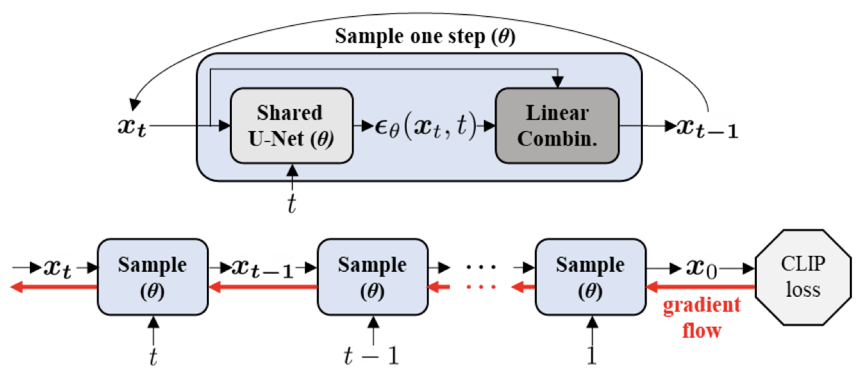
Figure 1. Gradient flows during fine-tuning the diffusion model with the shared architecture across t
Forward Diffusion and Generative Process
Kwon et al
Deterministic Diffusion Processes
The deterministic processes are formulated as follows:
$x_{t+1} = \sqrt{\alpha_{t+1}}f_\theta(x_t, t) + \sqrt{1 - \alpha_{t+1}}\epsilon(x_t, t)$
$x_{t-1} = \sqrt{\alpha_{t-1}}f_\theta(x_t, t) + \sqrt{1 - \alpha_{t-1}}\epsilon(x_t, t)$
Fast Sampling Strategy
To expedite the sampling, a ‘return step’ is introduced along with a strategy to use fewer discretization steps. This accelerates training without significantly compromising the identity preservation of the object in the image.
Detailed mathematical derivations and more comprehensive analyses can be found in the supplementary sections of
Experimental Setup and Procedure
Our method is intended to be used given a setup as follows. We have a set of images from the source domain, \(\{x_i\}_{i=1}^{n}\), out of which we have labels \(\{y_i\}_{i=1}^{n'}\) for a subset of them, where \(n' << n\). For simplicity, we are dealing with a binary classification task with 0-1 labels. We now want to classify test images from the target distribution, \(\{x^t_i\}_{i=1}^{m}\) (\(m << n\)). We also have a text description of the target distribution, \(T_{target}\) (a short prompt that captures how the source and target domains differ; for example, if the source domain is images in the summer and the target domain is images in the winter, \(T_{target}\) could be “winter”).
We now use the images from the source domain \(\{x_i\}_{i=1}^{n}\) to train a diffusion model and use DiffusionCLIP fine-tuning to generate an image \(x'_i\) from each labelled source image \(x_i\) driven by \(T_{target}\). Thus, we have created a new training dataset with the target distribution \(\{(x'_i, y_i)\}_{i=1}^{n'}\).
Now, we use supervised learning to train a model on the \(\{(x'_i, y_i)\}_{i=1}^{n'}\) pairs and subsequently classify the test images \(\{x^t_i\}_{i=1}^{m}\). The idea is that by shifting the distribution of training data to match that of the test data using just the text description of the target distribution, we can achieve a model that generalizes well to the target domain even in the regime of limited labelled data and target domain images without having to explicitly learn the target distribution.
Experiment and Results
Problem set-up
We run a simple experiment to show the power of domain adaptation using our method in this setting. We consider a gender classification problem on CelebA dataset with test domain being different from the train domain.
Our train domain is original CelebA images while our target domain is the same images but in the “sketch” style. The “sketch” style images were generated by the same method (DiffusionCLIP) by editing the original CelebA images on the test set. This style transfer doesn’t change the face identity (including gender, which is of our interest for the given task), so we keep all the labels unchanged.
We have a training set of size 1,200 images and test set of size 300 images (mainly for computation reasons). Our data comes from publicly available CelebA dataset with binary attributes (including the gender attribute of interest)
We use a simple CNN architecture for gender classification - three convolutional layers with increasing filter depth (32, 64, 128), each followed by a max pooling layer that halves the image dimensions, followed by 2 fully connected layers with sigmoid activation. Our experiment is ran for demonstrative purposes for the most part and does not require complex architectures. The training size of 1,200 images is additionally hinting at the necessity to scale the model complexity down for the purposes of our experiment. Our objective function is binary cross-entropy loss.
Experimental pipeline
We run the following experiments to confirm our intuition about the method’s effectiveness:
- Experiment 1
- Training set (1,200 labeled images) - original CelebA images
- Test set (300 labeled images) - “sketched” images
- We train CNN on plain CelebA images and evaluate on a shifted test domain. We use the plain CelebA test domain as a performance benchmark. We expect this model to do worse on the “sketched” test set than on the original one.
- Experiment 2
- Training set (1,200 labeled images) - adapted images. Original train images adapted to the “sketch” style using the method described in the subsection below.
- Note: We keep the number of images in the train set the same as in the experiment above (e.g., we create new train images and delete the original ones instead of augmenting the data) for the clarity of the experiment. In practice, one can combine images from both domains for learning.
- Test set (300 labeled images) - “sketched” images.
- We train the CNN on the “sketched” images now and evaluate the performance on both “sketched” and plain test sets. We expect this model to do better on the “sketched” test set which is our initial goal.
- Training set (1,200 labeled images) - adapted images. Original train images adapted to the “sketch” style using the method described in the subsection below.
Domain adaptation method
To edit our images from the plain CelebA distribution to the target “sketched” distribution, we use the method proposed in DiffusionCLIP
Despite the sufficient computation cost savings by using the DDIM process, transforming 1,500 images took more than 6 hours on a single NVIDIA GeForce RTX 3050TI 4GB GPU. Computation time is still the main drawback of using diffusion models for image editing and this is the main reason for us to limit the total sample size to 1,500 images.
Note: We use the same procedure for generating test images from “technically unknown” sketch domain and adapting the training set to this domain. This assumes the user perfectly identified the prompt which describes the target domain and used it to fine-tune the pre-trained diffusion model which is unrealistic in practice. We believe, however, that for simple prompts semantic similarity of the user prompt and the word “Sketch” would allow to get adapted images similar to the target domain because of the CLIP loss properties.
Results
Image Manipulation
Figure 2 shows examples of DiffusionCLIP fine-tuning applied to CelebA images, resulting in “sketched” images.
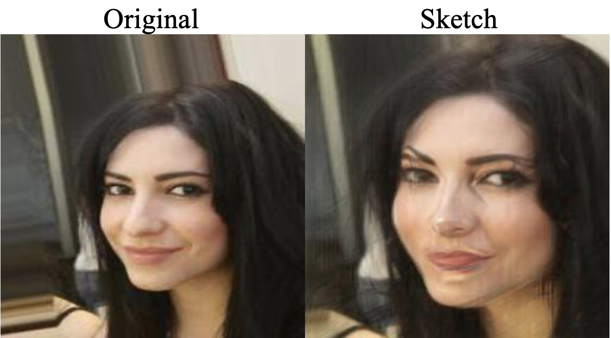
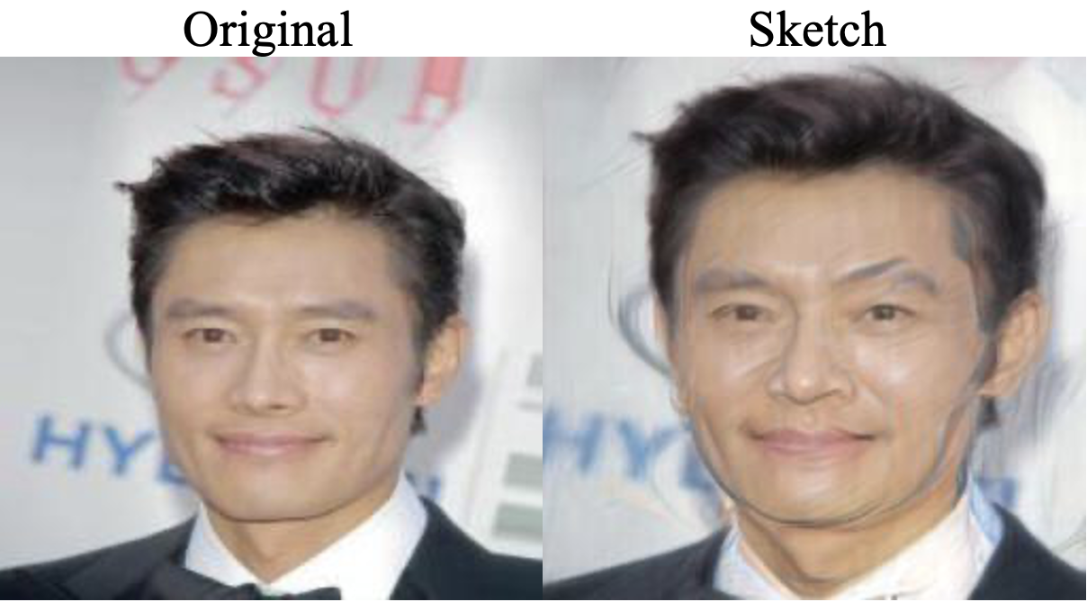
Figure 2. Examples of DiffusionCLIP fine-tuning.
Classification
Figure 3 shows the performance of the CNN trained on the original CelebA images and tested on images in the source domain as well as the target domain, while Figure 4 shows the performance of the CNN trained on the adapted images.
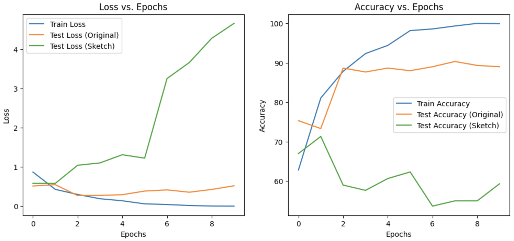
Figure 3. Performance of CNN trained on original CelebA images.
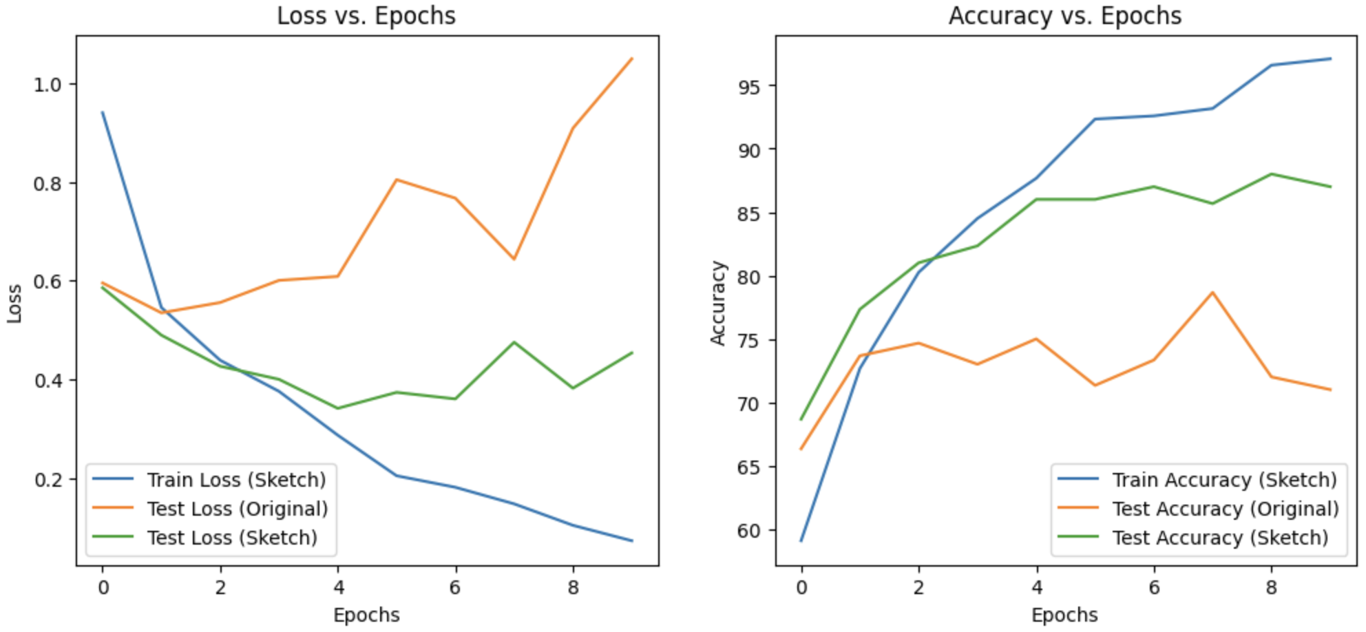
Figure 4. Performance of CNN trained on adapted images.
These results confirm our intuition that adapting our source domain to the target domain results in a non-trivial performance boost. We observe that for the initial few epochs, the performance for both the source and target domains is similar, but this gap increases as we train further. This tells us that initially, the model learns relevant “higher level” features that are present in both the domains since they are both related. However, for later epochs, the model overfits to the distribution of the training data which results in a large performance gap between the two domains. At this stage, the model is learning “lower level” features that belong to the source domain, which are different in the target domain. Thus, the performance on a shifted domain becomes worse as time goes on. If we train further, we expect to learn more lower level features of the source domain, which will enhance performance for a test set from the source domain but deteriorate performance for a test set from the target domain.
Conclusion
We have shown, with a simple binary classification experiment, that the proposed domain adaptation method using DiffusionCLIP fine-tuning leads to a significant performance boost when we have training and test data sampled from different but related domains.
Future work in this direction might include working with the h-space proposed in