Exploring Univariate Time Series Anomaly Detection using VAE's
In this blog post, we will take a deep dive into DONUT, a method that applies variational autoencoders to the problem of time series anomaly detection. We will begin with a overview of the original authors main ideas. Next, we will replicate some results, and perform new experiments to gain further insights into the properties, successes, and limitations of this method. Finally, we will run additional experiments that test extensions on the original formulation, and motivate future areas of exploration.
Introduction
Anomaly detection in time series data is a extensively studied field in academia, holding significant importance due to its wide-ranging applications in real-world scenarios. Time series are present everywhere, and the ability to detect anomalies is vital for tasks such as identifying potential health issues, predicting system failures, or recognizing regime changes in business operations. There are a wide range of methods that have been developed over the years in order to tackle this crucial yet challenging problem. Classical methods approaches rooted in statistics have long been employed, but in recent years, researchers have began to experiment with adapting deep learning techniques to achieve performance improvements.
The deep methods can generally be classified into distinct approaches. The first approach is forecasting, where the method attempts to learn the generating process of the series, and then classifies a point in the series as anomalous if the ground truth value deviates significantly from the predicted value. The second type of approach reconstruction. The models attempt to learn the generating process of the series in a latent space. The model then reconstructs the series, and uses a well designed reconstruction score in order to classify the series points as normal or anomalous. DONUT is an example of a method that falls into this category.
Problem Formulation and Background
Xu et al
We begin by defining what an anomaly means in the context of time series. Darban et al
Overview on VAE’s
Generative modeling refers to the objective of generating data from compact, low-dimensional representations. Representation learning can be a byproduct of generative modeling, where the generative model attempts to learn lower dimension representations of data such that inputs with similar high level features will be close to each other in the low dimension representation. Conversely, inputs that have dissimilar features will be far away from each other in the lower dimension representation space. These properties imply that the representation learner learns a good representation of the data that captures as much distinguishing information as possible. VAE’s achieve this through a two step process. Given an input x, an encoder is learned that maps the the input to a latent space, and then a decoder takes the latent space representation and maps it back up to the original feature space. The key property of VAE’s is that they can attempt to enforce a specific distribution in the latent space, such that we can sample from it and generate real looking outputs. The goal is to learn a model \(P_{\theta}(x) = \int p_{\theta}(x | z) p_z(z)dz\), where x are the inputs and z is a random variable in our latent space. In DONUT, and in most other VAE methods, \(p_{\theta}(x | z)\) and \(p_z(z)\) are chosen to be gaussian. Given this model, we would like to find the parameters that maximize the log likelihood \(log P_{\theta}(x)\). This is often an intractable integral to solve or approximate, so a trick called importance sampling is used. We can rewrite the integral as
\[P_{\theta}(x) = \int p_{\theta}(x | z) p_z(z) \frac{q_z(z)}{q_z(z)}dz\]where \(q_z(z)\) is a distribution we know how to sample from. Now, we rewrite this expression as an Expectation
\[E_{z \sim q_z}[p_{\theta}(x | z) \frac{p_z(z)}{q_z(z)}]\]We can now use monte carlo integration to estimate this expectation. This estimation will be inefficient to estimate with the wrong choice of \(q_z\). It turns out that
\[q_z(z) = p_{\theta}(z | x)\]is the optimal choice for \(q_z(z)\), and because this distribution might be hard to sample from, we use the variational inference trick where we find an approximation to this distribution by minimizing the objective
\[J_q = KL(q_{\psi}(z | x) || p_{\theta}(z | x))\]Thus we can now define an objective to be minimized that is fully parametrized by \(\theta\) and \(\psi\).
\[J_p = -log E_{z \sim q_{\psi}(z | x)}[p_{\theta}(x | z) \frac{p_z(z)}{q_{\psi}(z | x)}]\]The monte carlo estimate of this expecation produces a baised estimation of \(\theta\), so instead of optimizing the objective directly, we optimize a lower bound of the negated objective. Using Jensen’s inequality and expanding out the log terms, we know that
\[-J_p \geq E_{z \sim q_{\psi}(z | x)}[log p_{\theta}(x | z) + log p_z(z) - log q_{\psi}(z | x)] = E_{z \sim q_{\psi}(z | x)}[log p_{\theta}(x | z)] - KL(q_{\psi}(z | x) || p_z(z))\]This expectation lower bound is known as the ELBO, and is the surrogate objective that VAE’s optimize in order to learn good encoders and decoders.
DONUT
The key goal of DONUT is to take a series with normal data and potentially anomalous data, learn how to represent the normal features of the series, and then use these representations to compute a reconstruction probability score. Intuitively, if the method learns to represent normal inputs well, an anomalous input will have a low chance of being well reconstructed, and thus will have a low reconstruction probability. The challenge is that in order for the method to work really well, it is important that the method does not attempt to learn good representations for anomalous data. Xu et al
Where \(\alpha_w\) is 1 when \(x_w\) is not an abnormal point, and 0 when \(x_w\) is abnormal. \(\beta = (\sum_{w = 1}^W \alpha_w) / W\). We will take a deep dive into this modified elbo through empiricall experiments and by considering what role each term in the objective plays in both the learning of the latent space, and performance.
The authors also introduce two innovations that serve to improve performance, something we will reproduce in our experiments. The first innovation is markov chain monte carlo imputation of the missing points. The authors hypothesize that during testing, the presence of missing points in a given sample window might bias the reconstruction of the window, and thus affect the reconstruction probability, so they introduce iterative generation of normal points that can replace the missing points. Additionaly, the authors implement “missing point injection”. Before each training epoch, they inject missing points into the training samples by randomly selecting a subset of training sample points and removing the points (setting their values to zero). Note that the original samples will be recovered after the epoch is completed. They claim that missing point injection amplifies the effect of M-ELBO by forcing DONUT to learn the normal representation of data in abnormal windows. It certainly helps to improve performance, and we will perform a more thorough emperical analysis on both injection, and the \(\beta\) term in the M-ELBO.
The authors formulate the reconstruction probability as follows. They begin with the expression
\[p_{\theta}(x) = E_{p_{\theta}(z)}[p_{\theta}(x | z)]\]The authors claim that this does not work well emperically, and thus choose to use \(E_{q_{\phi}(z | x)}[log p_{\theta}(x | z)]\) as the reconstruction probability score. If the negation of these scores exceed a given threshold, the point will be classified as an anomaly.
We now describe the model structure of DONUT. The encoder \(q_{\phi}(z | x)\) is represented by a deep fully connected net that maps x to a lower dimension feature space. Then there are two readout heads that map the learned features from the net to a mean and variance, which we will denote \(\mu_z\) and \(\sigma_z\). We can then sample \(z\) from \(N(\mu_z, \sigma_z)\). The decoder \(p_{\theta}(x | z)\) is represented by a deep fully connected net that maps a latent variable \(z\) to a larger feature space. There are then two readout heads that map the learned features to a mean and variance, which we will denote \(\mu_x\) and \(\sigma_x\). We can then sample \(x\) from \(N(\mu_x, \sigma_x)\)
Experimental Setting and Evaluation
Before we lay out the experimental findings and their implications, we begin by briefly describing the datasets used and their characteristics, model architectures, training, and the metrics used for evaluation. We will use three datasets for experimentation, two of which come from the repository of the original paper. The first dataset is called “cpu” and is a series representing some cpu related kpi sampled every minute. The second dataset is called “g” and is also sampled every minute. The third dataset is air temperature time series from CIMIS station 44 in Riverside California, sampled at hourly intervals in the month of March from 2009 to 2019. The dataset did not come with time stamps. These series are all mostly normal, with few anomaly points. This makes the problem more challenging and interesting.

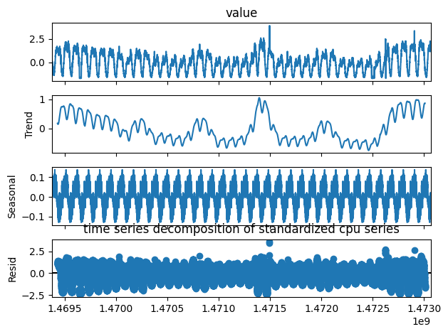

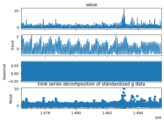

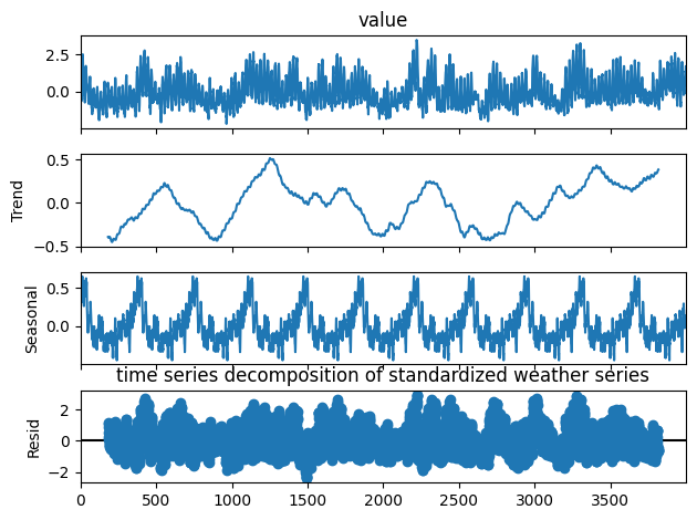
The cpu time series shows clear seasonality, and has an anomaly ratio of .015. The second series has much less clear seasonality, an anomaly ratio of .06, and is generally less smooth than the first series. This allows us to test the robustness of DONUT on a series that showcases less obvious seasonality, and draw some insights and comparisons on performance on series with relatively different smoothnesses. The weather series also displays clear seasonality and is smoother than the second series, but it differs from the other two series in that there are no anomalies in the training data. Thus, DONUT must learn to detect anomalies by training on purely normal data.
We create the training and testing data as follows. We begin by standardizing both the training and testing splits in order to represent all of the series on the same scale. We then set any missing values in the series to zero. Finally, we perform slide sampling in order to turn the series into windows of length \(W\). For each window, we will be predicting whether the last value in the window is an anomaly or not. We use a window size of 120 for the first two datasets which means our windows encapsulate two hours of information. For the weather dataset, we use a window size of 24, so each window encapsulates a day of information.
We will use the same metrics described by Xu et al
For our experiments. We will use fairly small and simple architectures. The baseline VAE in the paper is done using fully connected networks, and so we will use a fully connected network with depth two. We also experiment with CNN VAE’s, and in order to try and compare performance with the fully connected VAE encoders and decoders, we also use a CNN with two layers. We perform experiments on behavior when the latent dimension is increased, and needed to double the width and depth of the fully connected VAE in order to allow for training to converge.
Reproducing Results and Establishing Baselines
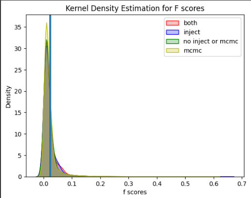
Xu et al
| Configuration | avg best f score over 10 runs |
|---|---|
| both | .642 |
| just inject | .613 |
| just mcmc | .5737 |
| neither | .588 |
Next, we run DONUT with the baseline configurations for each of our three datasets. We randomly sample a third of the training data and plot the selected samples mappings in 3-d z space. We also plot the predicted anomaly points by the model with the highest f score over the 10 runs for each of the three datasets.
| Dataset | avg best f score over 10 runs |
|---|---|
| cpu | .642 |
| g | .881 |
| weather | .996 |
Xu et al

They noticed that the latent space was spread out according to time of the day, as time of the day likely encoded a large amount of information about the shape of the series. We did not notice such a phenomenon in our experiments. This is likely the result of a difference in experimental setting, but could also be the result of the local variation within the seasonal data, and the fact that similar shapes occur all over the series irrespective of time. We see that on the second datset, DONUT learned to classify many troughs in the series as anomalous. It was able to detect both global anomalies, as well as contextual and seasonal anomalies, as seen by its ability to detect sudden flat shapes in the series and sudden spikes in the unsual places.

The performance on the third datset is quite suprising. Given no anomalous data in the train set, DONUT was able to achieve a .996 average best f score on the testing data. This highlights DONUT’s ability to really learn the normal features of a series. Thus during testing, it was not able to reconstruct the anomalous parts of the series as well as the normal parts. While this result does not contradict the claim that it is important to train on both normal and anomalous data, it certainly suggests that there is still value on learning purely normal qualities of the data. M-ELBO does not fully remove learning of anomalous qualities of the data in the latent space, which could lead to unexpectedly high reconstruction probability scores on anomalous testing data
Understanding The Latent Space
It is important that we gain further insights on the latent space, as it is the bottle neck of any VAE method. We will perform a variety of experiments that aim to fully uncover how each term in ELBO controls the characteristics of the latent space. We begin by first explaining the findings and claims of the original paper.
The authors claim that the number of dimensions in the latent space plays a huge role. A small dimension latent space would not allow you to capture enough information, and too big a latent space would cause DONUT to perhaps capture too much information, including anomalous representations. They found that latent dimensions between 3 and 10 typically produced good results. They next discuss how they believe each term in the ELBO contributes to the time gradient phenomena they observe. We restate the M-ELBO objective
\[E_{z \sim q_{\psi}(z | x)}[\sum_{w = 1}^W \alpha_w log p_{\theta}(x | z)+ \beta log p_z(z) - log q_{\psi}(z | x)]\]We can rewrite this objective as
\[E_{z \sim q_{\psi}(z | x)}[\sum_{w = 1}^W \alpha_w log p_{\theta}(x | z)+ \beta log p_z(z)] + H[z | x]\]Where \(H[z | x]\) is entropy. The authors claim that the first term, \(log p_{\theta}(x | z)\) requires the latent space to be able to reconstruct normal x well, thus it pushes latent representations of dissimilar x further away from eachother. The second term, \(log p_z(z)\), serves to encourage the gaussian shape in the latent space and thus encourages the latent space to not expand too much. However, we shrink the contribution of this term by the ratio of normal points in our training data. The entropy term encourages expansion of the latent space, as it is largest when the latent space encodes as much information as possible. This should happen when the latent represenations are as distinguishing as possible.
Effects of Changing the latent distribution
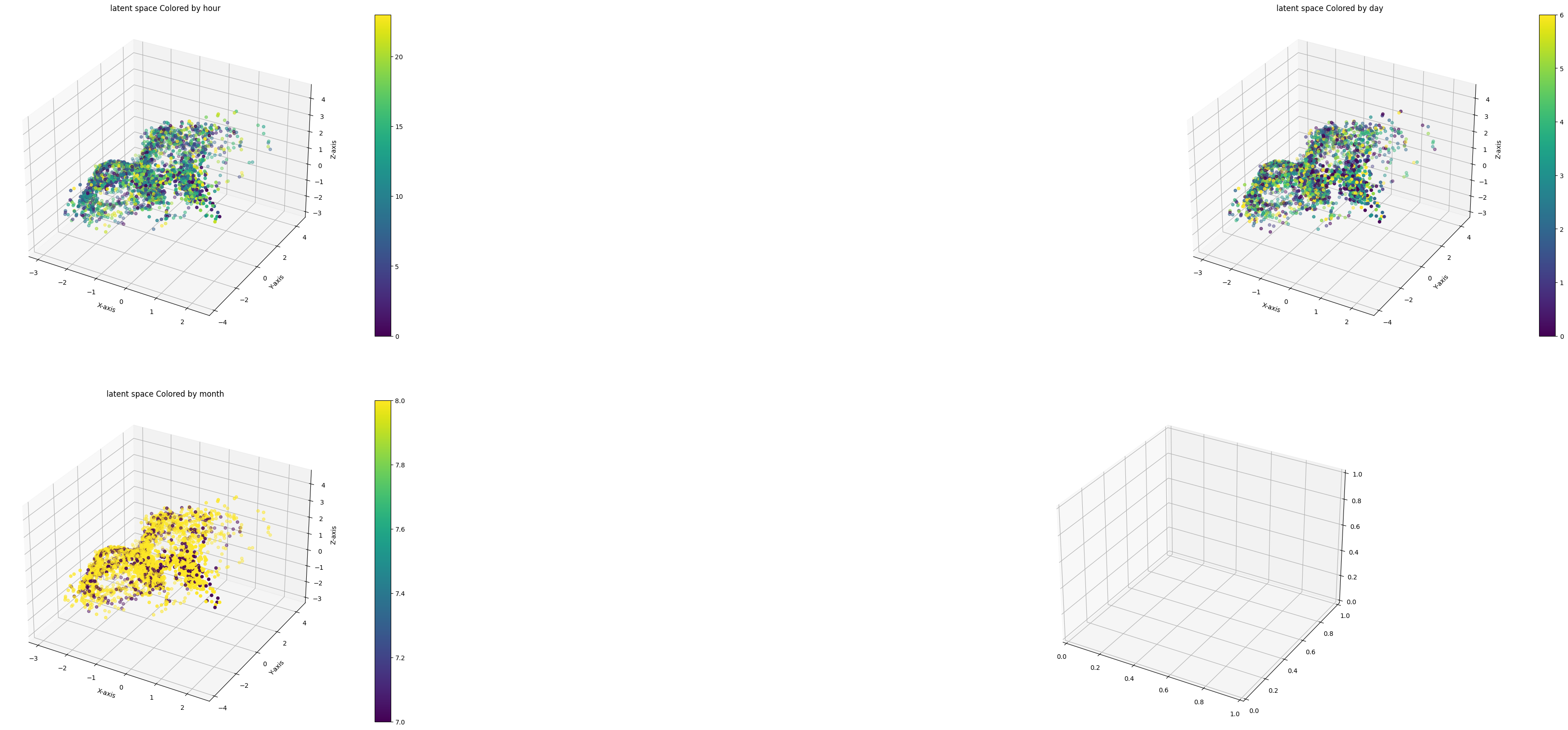
Most VAE methods traditionally represent the latent space as a mixture of gaussians, both for its simplicty, as well as its flexibility and ability to approximate many complicated distributions. What happens when we use other types of distributions? We will analyze what happens to performance and the shape of the latent space when we represent it as a mixture of Student-T distributions with 10 degrees of freedom. We hypthesize that replacing a mixture of gaussians with a mixture of any other symmetric distribution will not cause any profound differences in the shape of the latent space, at least in 3 dimensions, however, a symmetric latent space with fatter tails could lead to worse reconstruction performance. Consider \(P_{\theta}(x | z)\), where z is sampled from the latent space. With a fatter tailed distribution, we are more likely to sample a z that is further away from the mean of its distribution. This behavior can be beneficial for generative purposes but for reconstruction purposes, this behavior is likely detrimental and will lead to lower likelihoods that a given x came from the sampled z. We now analyze the empericall effects for all three datasets. For the cpu dataset, we notice that the latent space does not look drasticaly different, considering we only plot a random subset of it. We do however notice a performance dip.
| Latent Distribution | avg best f score over 10 runs |
| gaussian | .642 |
| t with 10 df | .593 |
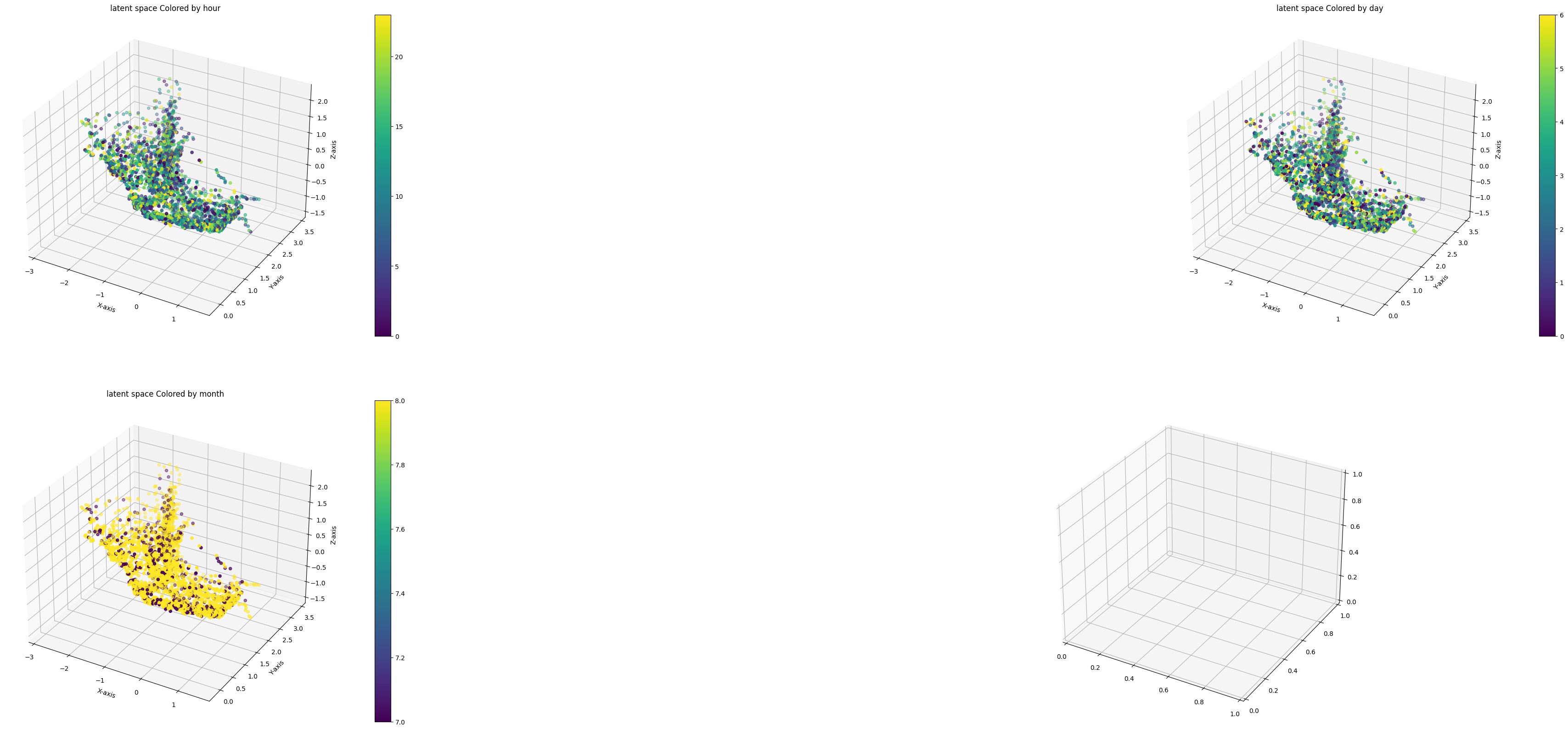
Similarly for the g dataset, we see a slight performance reduction, but a similarly shaped latent space.
| Latent Distribution | avg best f score over 10 runs |
| gaussian | .8809 |
| t with 10 df | .871 |
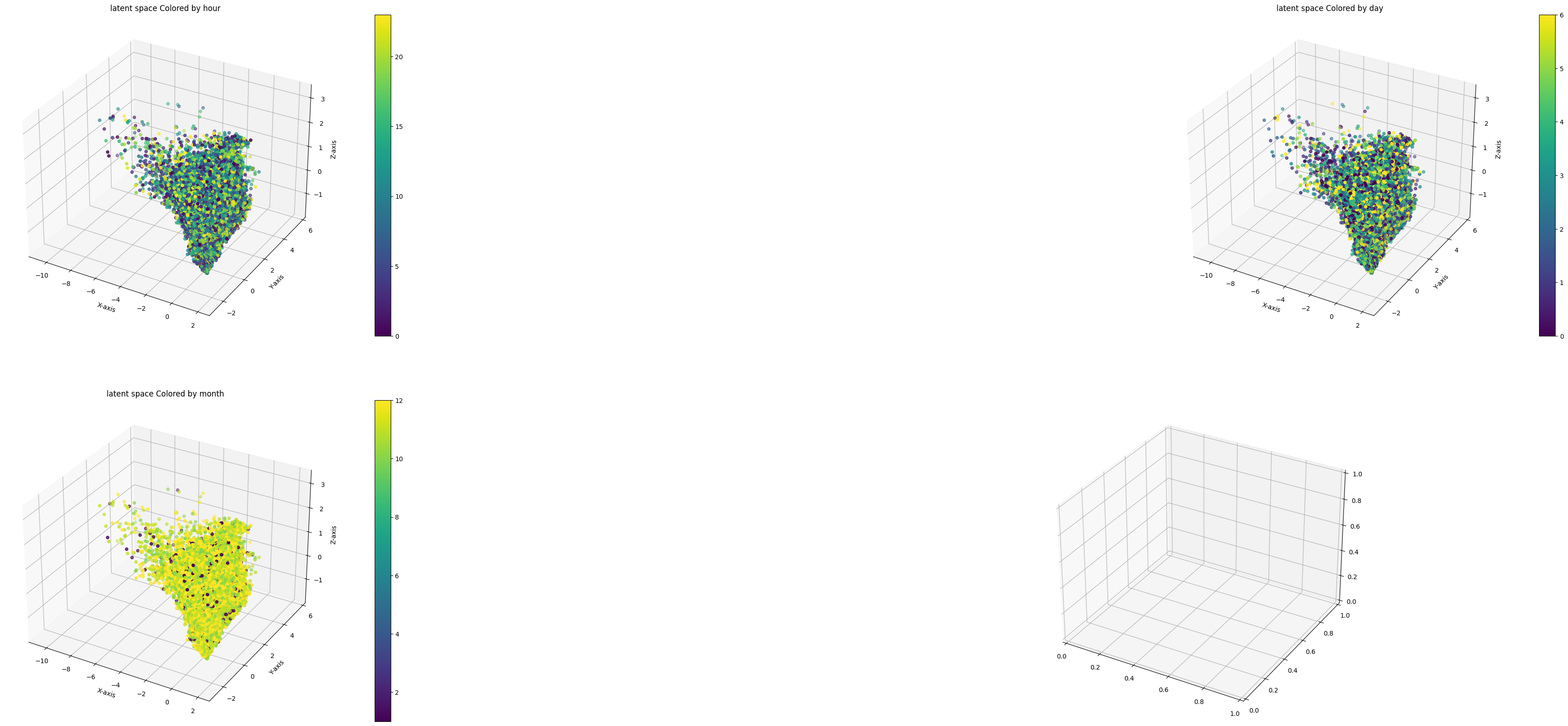

For the weather dataset, the performance reduction is negligible which suggests that the means of our learned latent space truly represent the normal patterns of the series. (Note that this dataset did not come with timestamps. Disregard any time colorations on latent space plots)
| Latent Distribution | avg best f score over 10 runs |
| gaussian | .996 |
| t with 10 df | .995 |

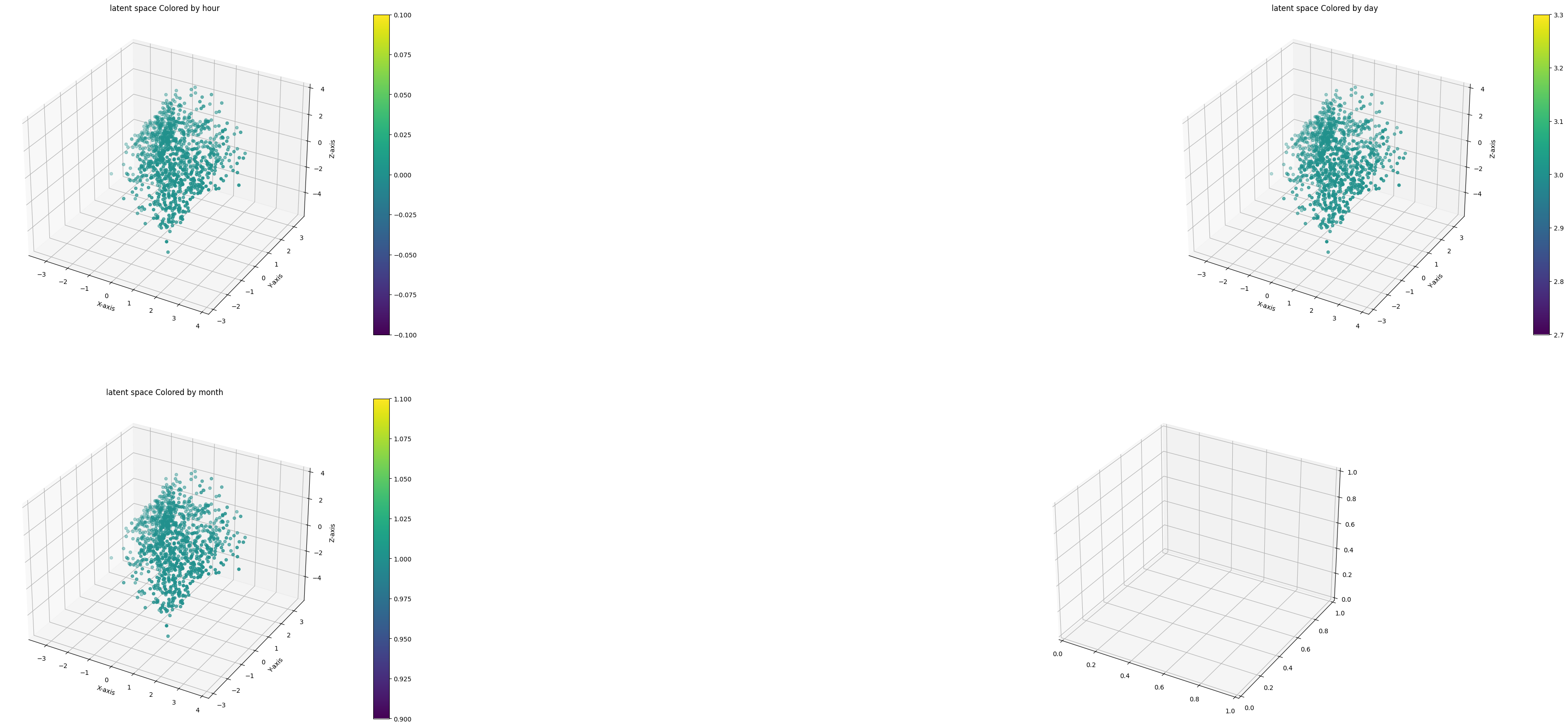
This brief analysis suggests that the gaussian distribution is truly a good adaptable choice for our latent space. It allows for some variability when doing generative modeling, but also allows for a more robust estimator of reconstruction probability.
Should we Scale the Entropy term in M-ELBO?
Xu et al
In our first experiment, we choose a reasonable choice for the weight of the entropy term. We will use \(\beta\) to weight both \(logP_{z}(z)\) and \(logq_{\psi}(z | x)\). Thus M-ELBO becomes
\[E_{z \sim q_{\psi}(z | x)}[\sum_{w = 1}^W \alpha_w log p_{\theta}(x | z)+ \beta log p_z(z) - \beta log q_{\psi}(z | x)]\]We can reformulate the M-ELBO in terms of the KL divergence to hypothesize what effects scaling \(logq_{\psi}(z | x)\) by \(\beta\) might have.
\[E_{z \sim q_{\psi}(z | x)}[log p_{\theta}(x | z)] - KL(q_{\psi}(z | x)^{\beta} || p_z(z)^{\beta})\]Using the power rule of logarithms, we can rewrite this objective as
\[E_{z \sim q_{\psi}(z | x)}[log p_{\theta}(x | z)] - \beta KL(q_{\psi}(z | x) || p_z(z))\]Thus we have essentially applied shrinkage to the KL divergence between the prior and the posterior based on the amount of abnormal data in our training data. This would perhaps encourage the latent space to look more gaussian, such that the prior probability dominates the posterior probability in order to increase the M-ELBO lower bound. Thus we can hypothesize that our latent space will perhaps experience shrinkage. This would certainly be undesired behavior if our goal is to expand our latent space and allow for more distinguishing latent space represenations while keeping some form of structure.
We now analyze the emperical results. We first analyze the effects on the cpu dataset. There does seem to be signs of shrinkage in the latent space when it is weighted, however there is no clear absolute shrinkage or expansion. The shape is certainly different, and it seems like the latent space expanded in the negative direction in the second dimension of the latent space, and shrunk in the positive direction. We also observe a performance increase.
| avg best f score over 10 runs | |
| Unweighted Entropy | .642 |
| Weighted Entropy | .665 |


On the g dataset, we can certainly see a differently shaped latent space. We notice that the third dimension of the latent space expanded, while the first and second dimensions showed some level or shrinkage compared to the baseline. We do see a slight reduction in performance compared to the baseline
| avg best f score over 10 runs | |
| Unweighted Entropy | .8809 |
| Weighted Entropy | .875 |

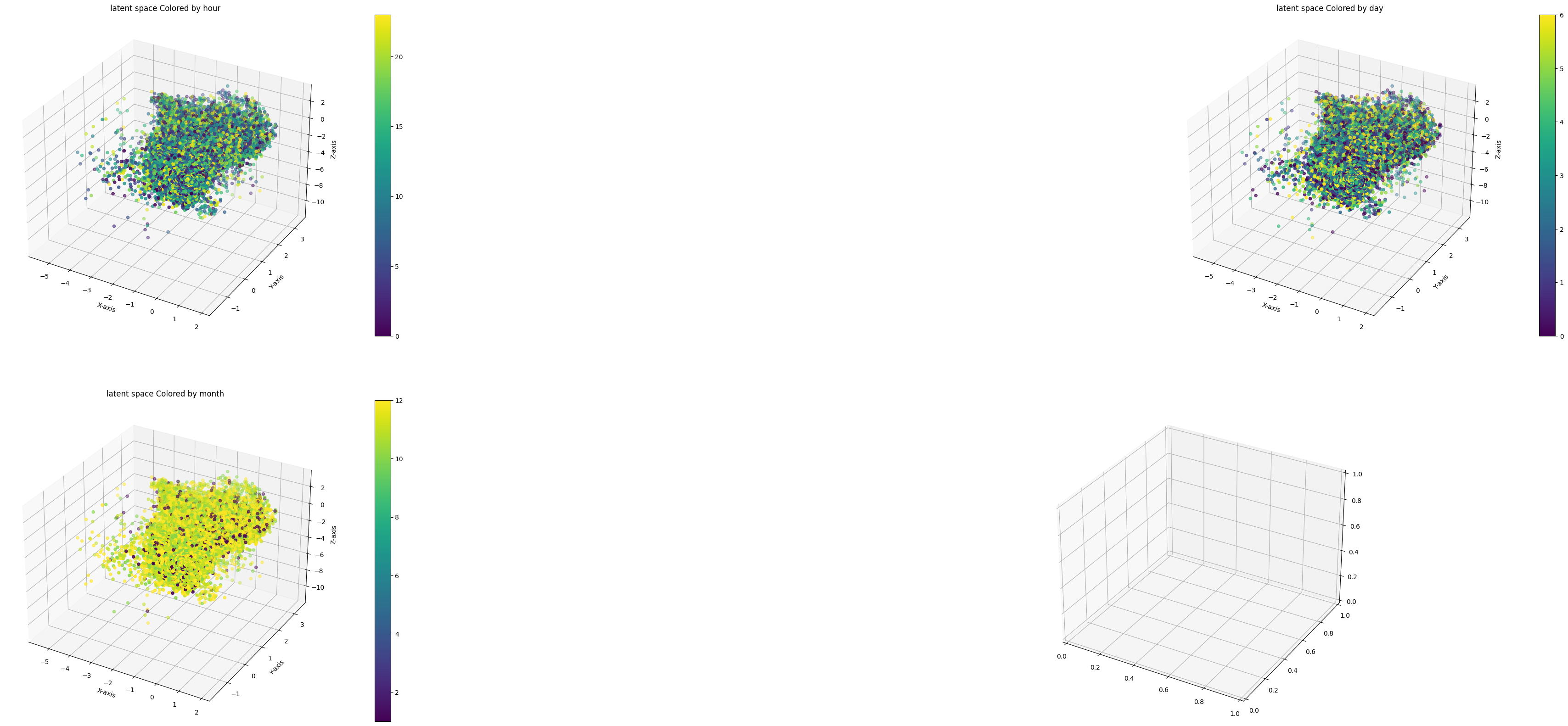
Finally, for the weather dataset, we also see that weighting the entropy term did not lead to absolute expansion or shrinkage of our latent space. We observe shrinkage in the third dimension of the latent space, slight shrinkage in the first dimension, and slight expansion in the second dimension. We also observe a slight performance dip.
| avg best f score over 10 runs | |
| Unweighted Entropy | .9967 |
| Weighted Entropy | .9928 |

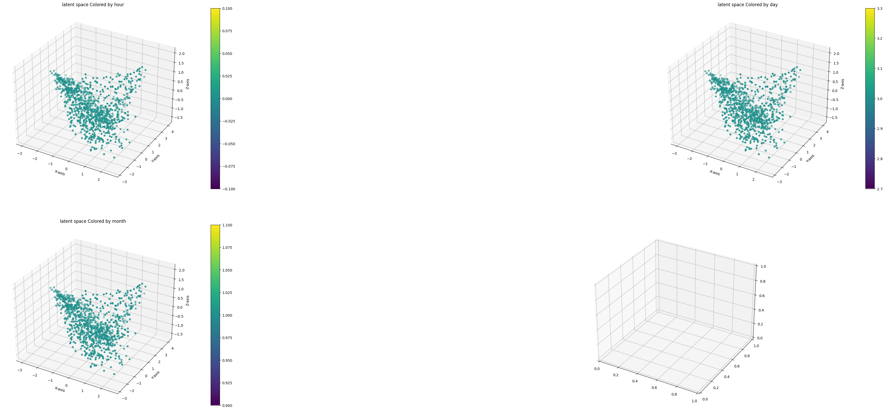
These results suggest that weighting the entropy term can lead to shrinkage of the latent space. It certainly lead to different latent space shapes, where we observed expansion in some dimensions and shrinkage in others. There are also no conclusive results in its affects on performance, as we saw improved performance in one dataset and decreased performance in the other two.
We will now perform a more general experiment on the effects on weighting the entropy term with the cpu dataset. Instead of weighting the entropy term with \(\beta\), we will try different weights between 0 and 1 and observe the effects. We increased the capacity of our VAE network, so we rerun the experiments on weighting entropy with \(\beta\) and not weighting entropy in order to have a valid comparison of results.
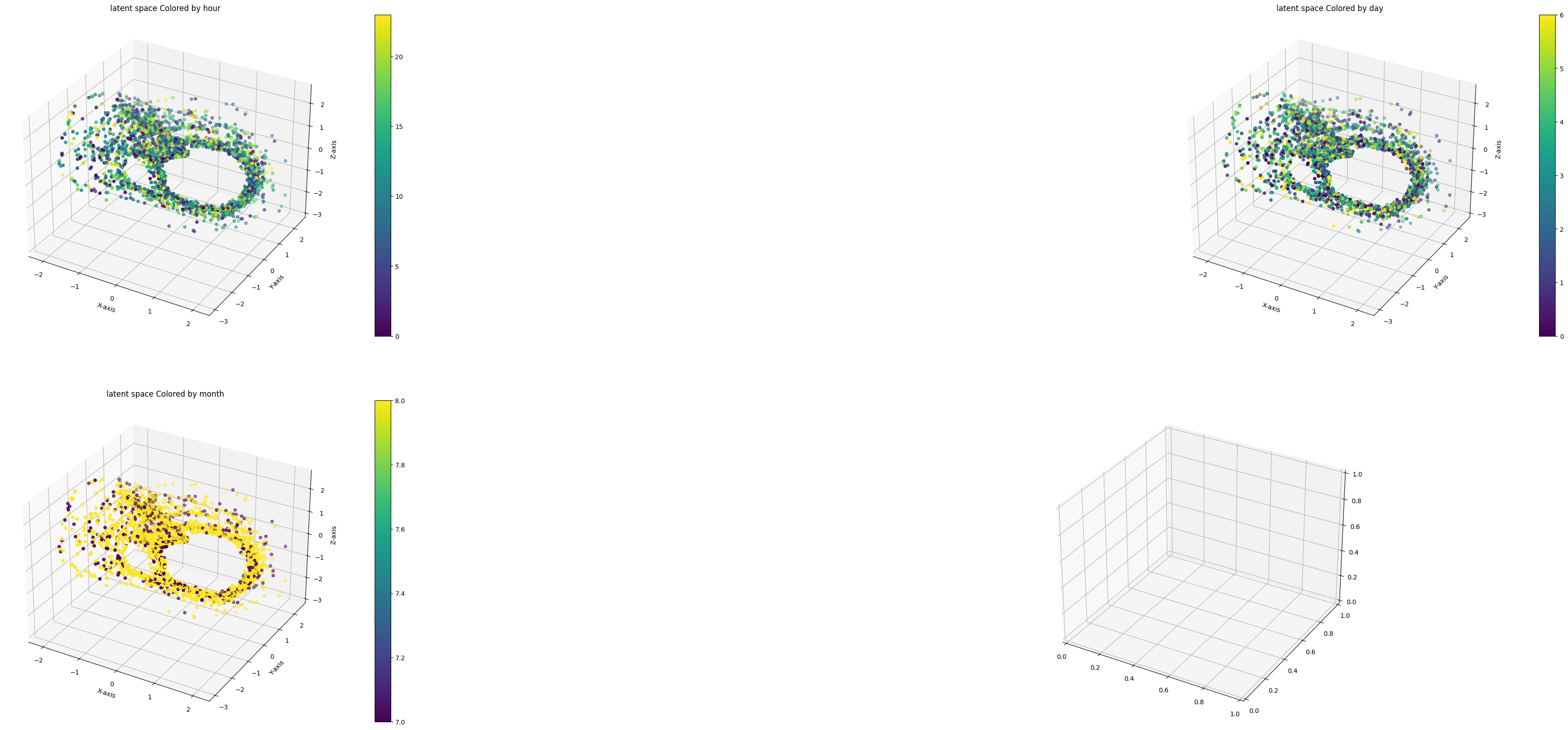
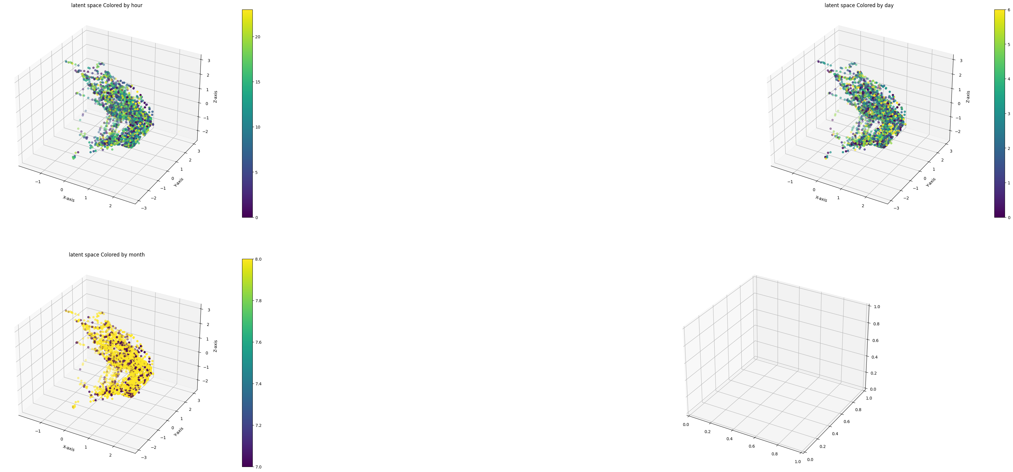
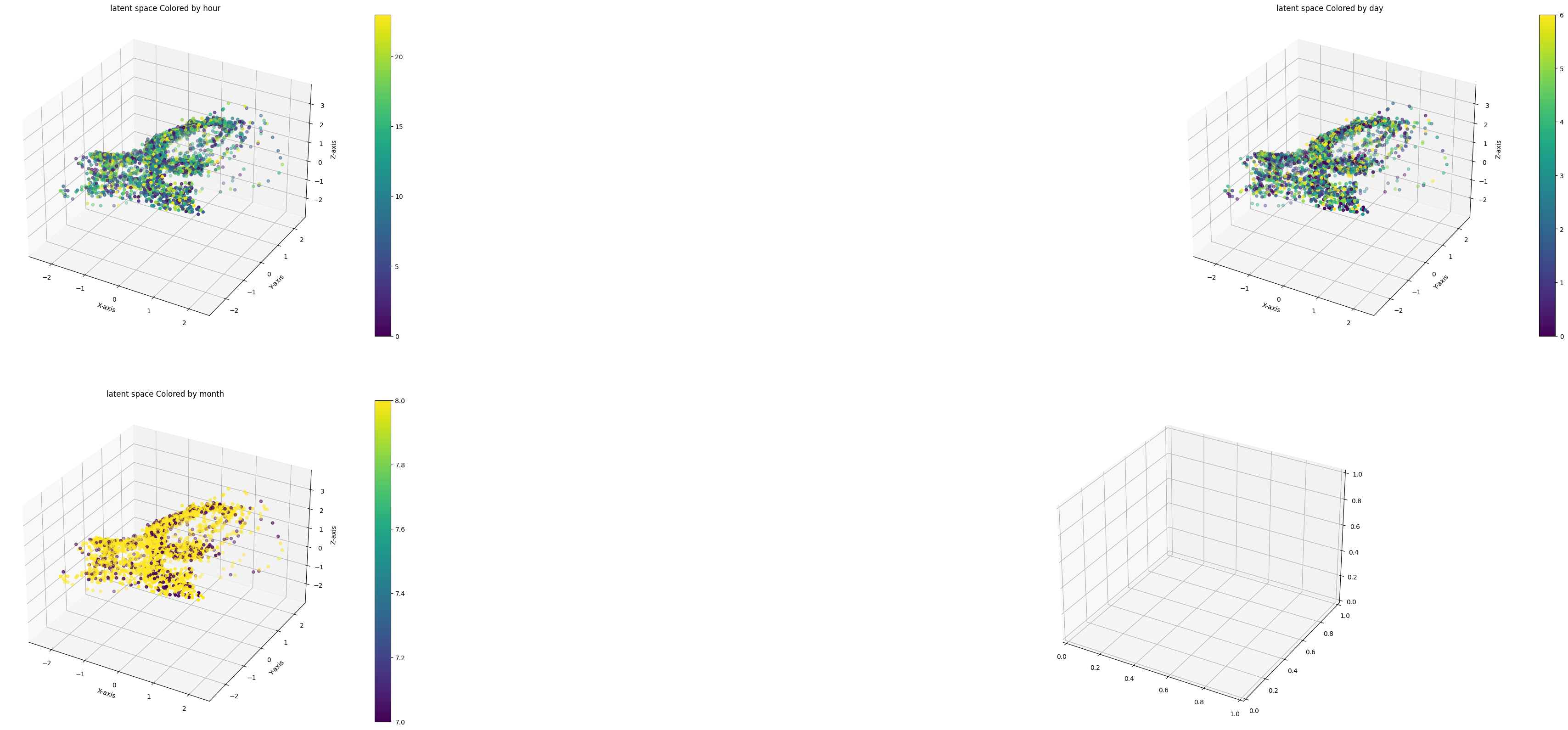
When the entropy term is weighted by zero, we notice a very speherically shaped latent space which looks like a unit gaussian ball. This matches up with a quick evaluation of the elbo. There is no more reshaping of our latent space by the entropy term, and thus DONUT learns a latent space that matches up with the gaussian prior. With a weight of .2, we again see a circular latent space, however there is more deviation from a spherical shape. We continue to see this phenomenon of deviating from a spherical shape when the weights increase. We also notice that the points become more clustered as the weights increase. There seems to be a level of shrinkage as the weights increase, but for weights equal to .8 and .9, we see the latent space expand again. These results indicate that it is unlikely that weighting the entropy term has any effect on expanding the latent space. Results even suggest that non zero weights can lead to shrinkage. However, weighting the entropy term certainly affects the shape of our latent space, and the ability of the VAE to learn representations that look less guassian.
The performance results provide some interesting insights, and can serve to motivate future areas of exploration. We see that performance is maximal when the weights are very low, or around .6 and .7. When the weights are low, the latent space is very constrained, and thus DONUT will learn learn purely normal representations of the data. As the weights increase, and the ability of DONUT to learn latent representations that deviate from purely guassian increases, we generally see consistently good performance that is comparable to the zero weight case. With weights larger than .8, we begin to see a dip in performance. With large weights, the latent space deviates the most from being gaussian shaped and perhaps begins to learn anomalous representations. This suggests a benefit to enforcing more normality and constraint on the shape of our latent space for the purposes of anomaly detection. This could mean not weighting the prior term by \(\beta\), or adding some additional terms to M-ELBO that somehow enforce the latent space to look more guassian.
| weight | avg best f score over 5 runs |
|---|---|
| 0 | .682 |
| .1 | .673 |
| .2 | .657 |
| .3 | .602 |
| .4 | .666 |
| .5 | .634 |
| .6 | .7 |
| .7 | .688 |
| .8 | .602 |
| .9 | .625 |
| 1 or unweighted | .64 |
| Beta weighted | .6 |



Empirical Exploration of the Effects of Beta and the Missing Data Injection Rate
We now perform analysis on exactly how \(\beta\) affects $p_z(z)$, both through experimenting with differing rates of missing data injection, as well as manually adjusting \(\beta\) and observing the results.
We restate M-ELBO in tems of the KL divergence.
\[E_{z \sim q_{\psi}(z | x)}[log p_{\theta}(x | z)] - KL(q_{\psi}(z | x) || p_z(z)^{\beta})\]As \(\beta\) decreases, the KL divergence increases. In order to decrease the divergence, the VAE should decrease the posterior probability, which could lead to a more spread out or non gaussian looking latent space, or rather one where we learn very distinguishing representations. As seen from our previous analysis, this might be undesired behavior for the purposes of anomaly detection. Performing automatic reduction of \(\beta\) by increasing the missing data injection rate could prevent DONUT from learning enough about the normal patterns in the training data, and thus performance will likely suffer if the injection rate gets too large.
We begin first by trying out \(\beta\) values between 0 and 1 in order observe the effects, and motivate adjusting the missing data injection rate.
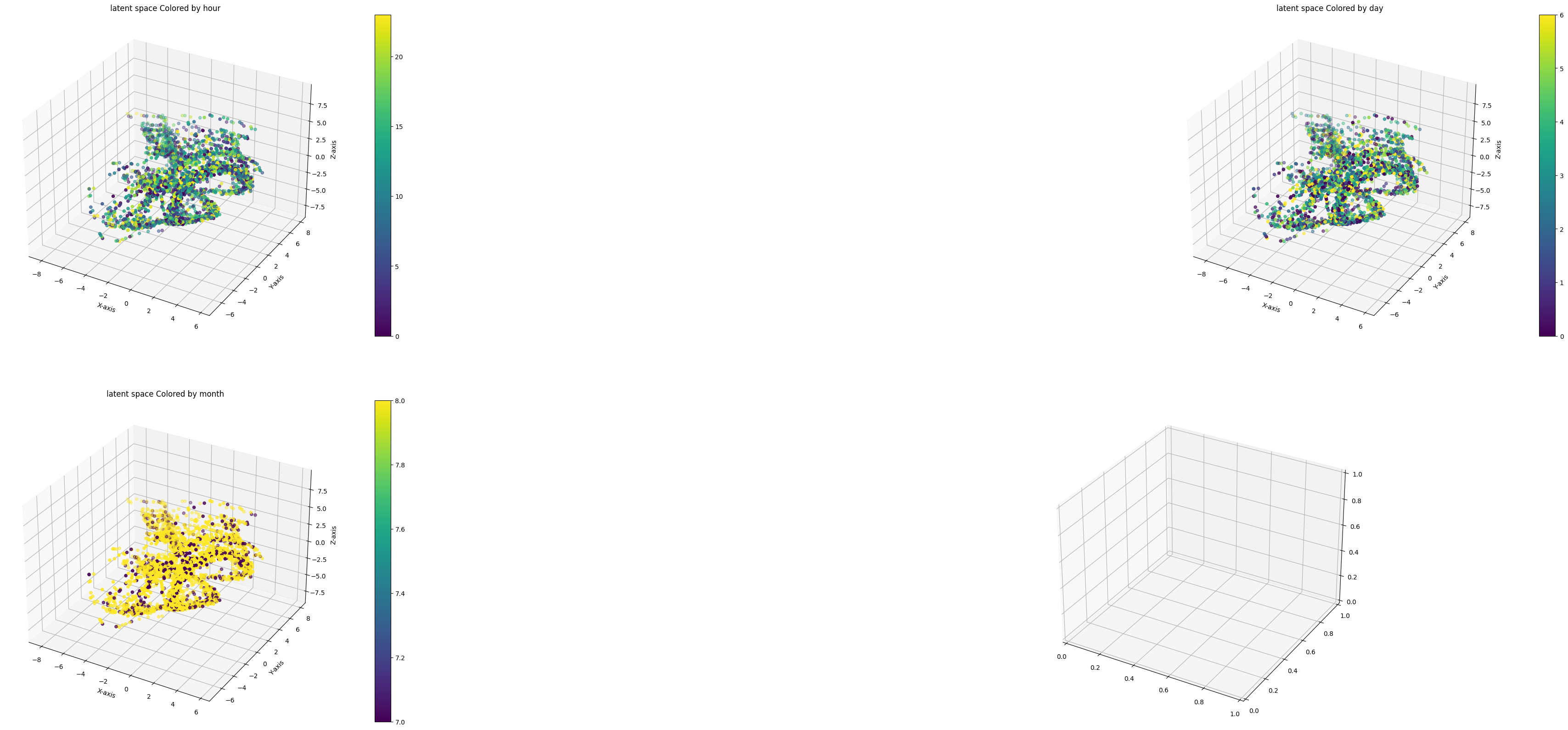
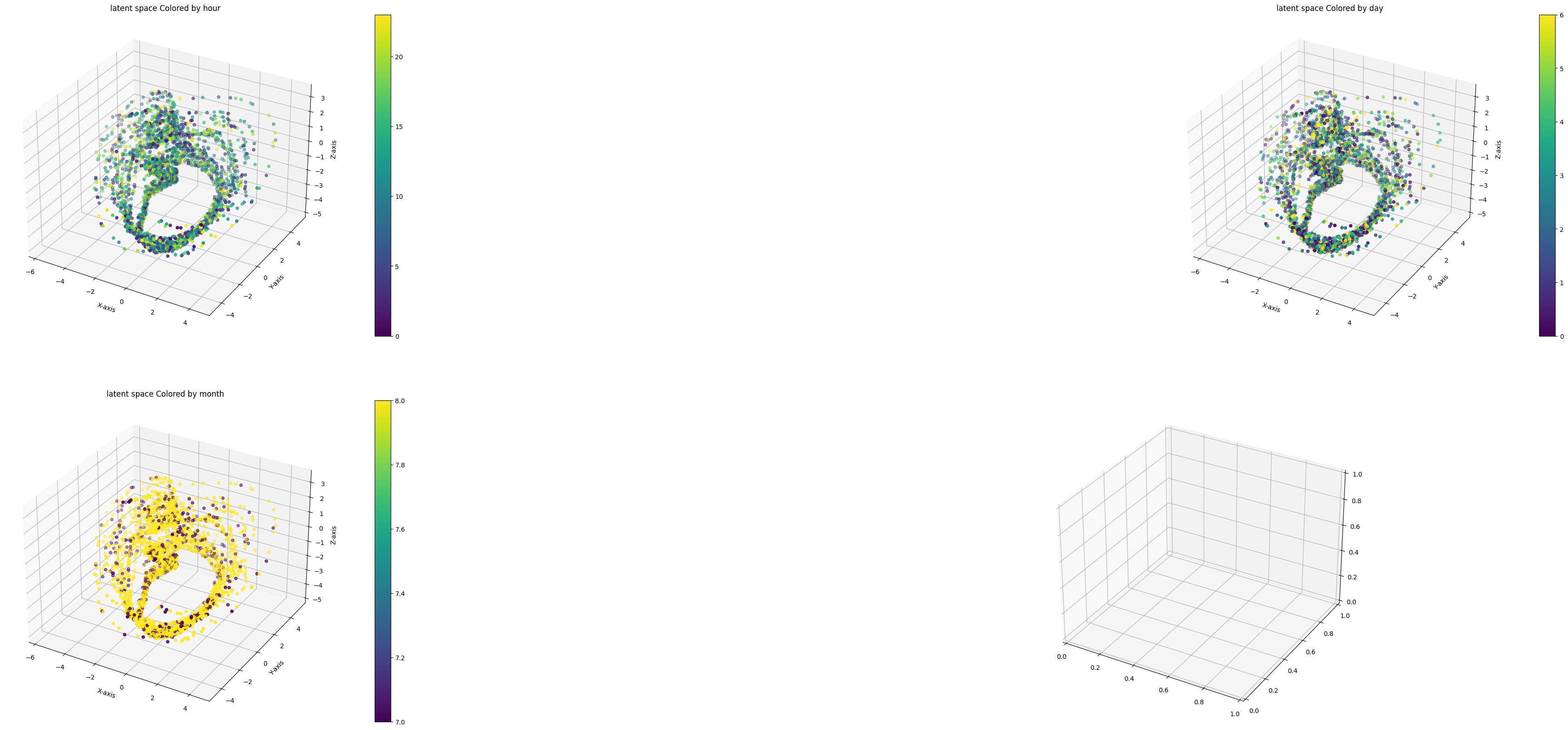
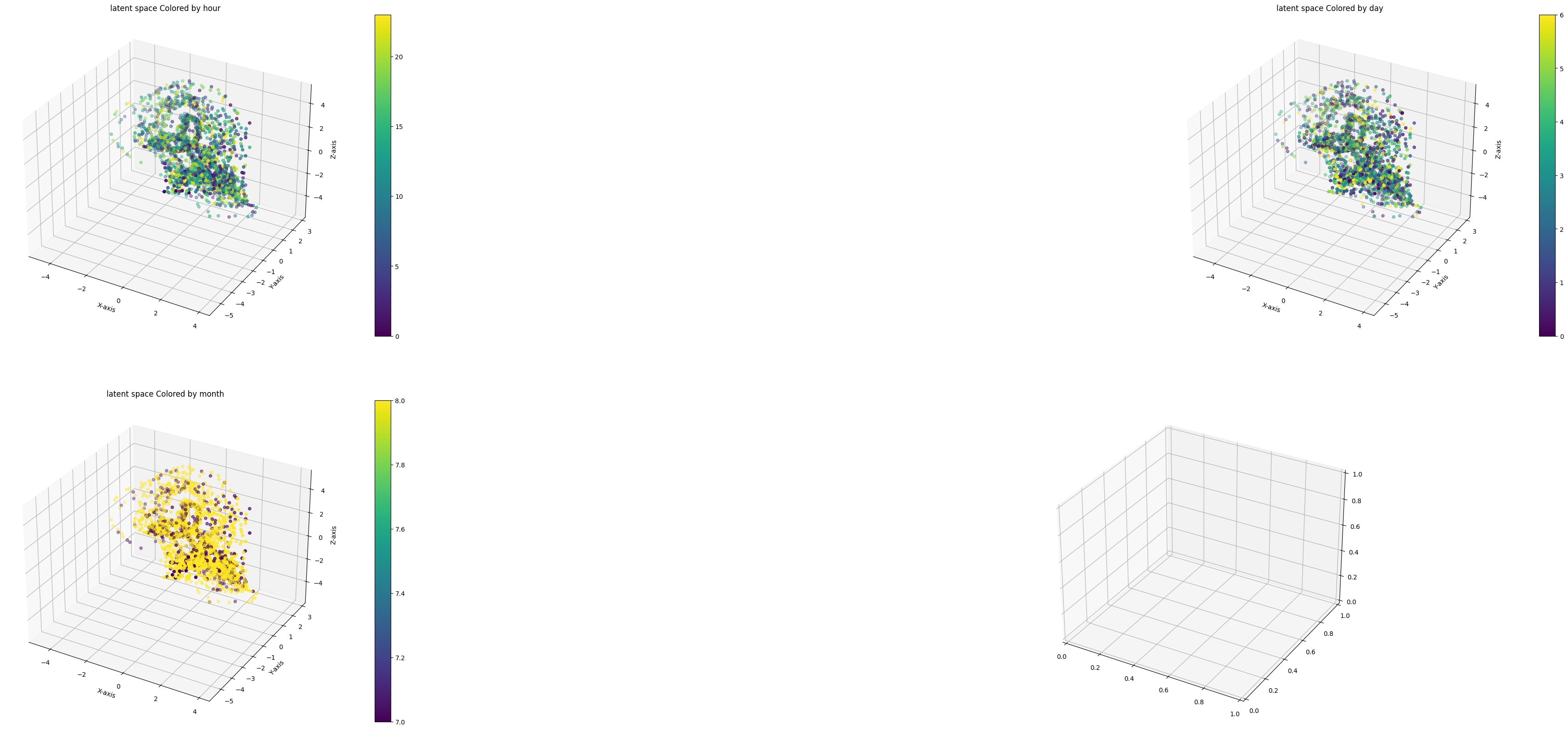
When \(\beta\) is set to to 0, we see that the latent space looks fairly compact and non spherical. At \(\beta\) between .1 and .4, we can see that the latent space is quite spread out, and displays some spherical properties, especially for \(\beta\) = .3. For \(\beta\) between .4 and .9, we can see that the sampled latent space begins to look more and more compact, yet there is still a reasonable spread in the latent space. There does not seem to be a clear relationship between the spread and shape of the latent space and perfomance, however, we note that the \(\beta\) that resulted in the highest performance was \(\beta\) = .3, whose latent space looks the most spherical. This again supports the notion that when the latent space looks more gaussian, anomaly detection is improved.
| Beta | avg best f score over 5 runs |
|---|---|
| 0 | .648 |
| .1 | .595 |
| .2 | .591 |
| .3 | .686 |
| .4 | .633 |
| .5 | .6 |
| .6 | .623 |
| .7 | .614 |
| .8 | .669 |
| .9 | .646 |
| 1 or unweighted | .64 |
| Beta weighted | .6 |

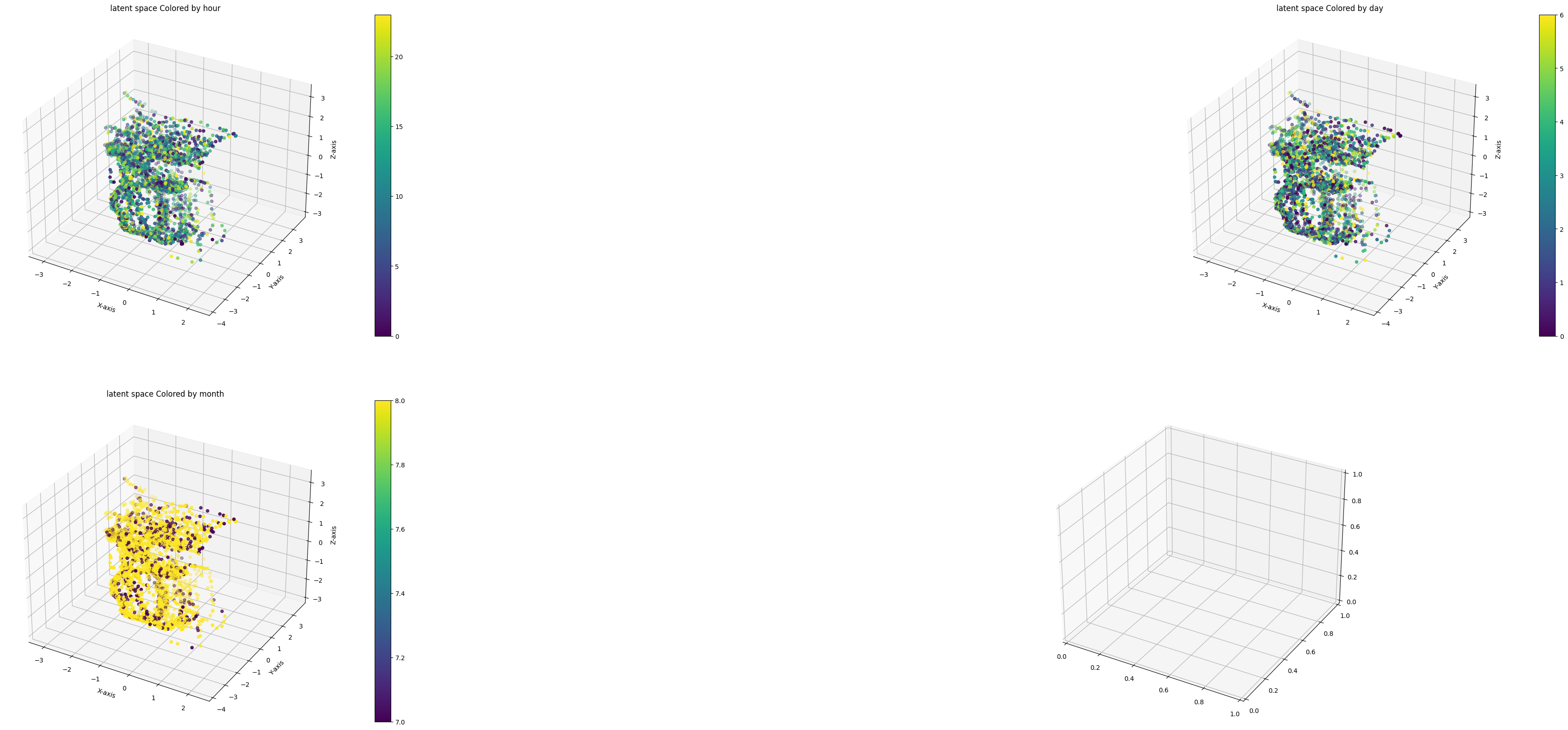

In our experiments on adjusting the missing injection rate, we saw a significant decrease in performance as the rate increased, even reaching an average best f score of .06 when the rate was .8. It is unclear from our experiments whether this is the result of training not converging, as we do observe high loss values, or simply bad performance of DONUT when a vast majority of the data is missing, which would be expected behavior. This is something that would need to be explored further
Improving VAE Architecture
For the purposes of simplicity, DONUT utilizes fully connected layers for both the encoder and the decoder. While these choices certainly produce decent results, perhaps we can implement architectures that can better utilize the temportal information encoded within each window. We explore using a one dimensional CNN for the encoder in DONUT. Perhaps CNNs are better able to learn representations that encode more temporal information within a sample window. In order to make the CNN network as comparable as possible with the fully connected network, we will only use two convolution layers. We apply a kernel size of 3, and a stride of 1. We also use max pooling to downsample the data.
For the cpu dataset, we observe significant performance improvements with the CNN architecture. We notice the detection of contextual anomalies, which are non obvious local deviations. The latent space looks fairly spherical, however there does not seem to be any noticeable time gradient behavior in the latent space, despite the improved ability of the encoder to take advantage of temporal information.
| Architecture | avg best f score over 10 runs |
| 2 layer CNN | .714 |
| 2 layer fc | .642 |


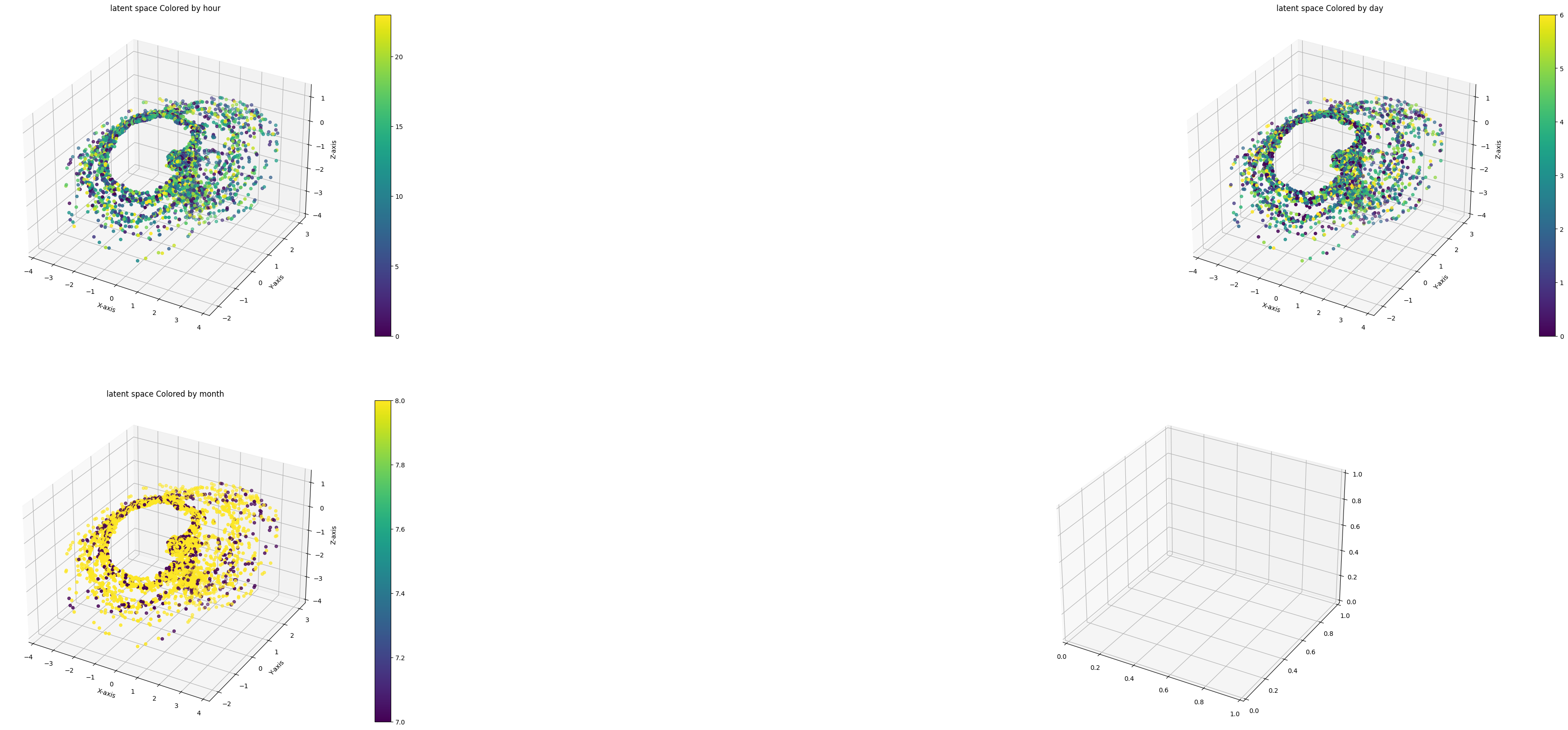
We did not see this same performance improvement in the other two datasets. Additionally, we struggled to achieve stable training on the weather dataset, and so further work needs to be done to achieve convergence in order to perform evaluations on the efficiacy of CNNs with that dataset. For the g dataset, we noticed a significant performance reduction. The difference between the performance on the cpu dataset and the g dataset could suggest that CNN architectures could lead to overfitting on less smooth time series. Looking at the plot of predicted anomalies seems to suggest this, as DONUT with a CNN encoder seems to predict that a larger number of the troughs in the g series are anomaly points, an indicator of potential overfitting to the series pattern.
| Architecture | avg best f score over 10 runs |
| 2 layer CNN | .824 |
| 2 layer fc | .881 |


This is an interesting area of exploration for DONUT. There are a variety of architectures such as RNN’s and transformers that have shown superior performance on time series data, and those could be adapted to this method to improve performance over both CNN and fully connected architectures.
Choosing Number of Latent Space Dimensions
For the purposes of plotting the latent space in our experiments, we chose to use use a latent space with dimension three. However, intuitively, and as shown in the paper, choosing higher a higher dimension latent space can lead to performance improvements.
We hypothesize that smoother series do not need as large a dimension in the latent space as series that display higher levels of roughness. Intuitively, in smoother series, the anomalies should be more “obvious”, while in less smooth series, rough behavior could be mistaken for an anomalous pattern.
We take a technique from smoothing splines, which are function estimates obtained from noisy observations of some data process. Smoothing splines enforce a roughness penalty on the function estimate, defined as such
We will use a finite difference estimate of this penalty on the standardized series to define a metric that can be used to describe the roughness/smoothness the series. Now that we have defined a metric describing the smoothness of a series, we can evaluate the best choice of number of latent dimension for series of differing levels of smoothness. In order to converge during training, we had to double the width of the fully connected VAE, and also double its depth.
| Dataset | Roughness Penalty |
|---|---|
| cpu | .061 |
| g | .598 |
| weather | .023 |
We begin with the cpu dataset. We notice that performance significantly increases when the latent space is 6 dimensions, but performance begins to drop off as the number of dimensions increases, which suggests overfitting.
| number of dimensions | avg best f score over 5 iterations |
|---|---|
| 3 | . 637 |
| 6 | .833 |
| 9 | .826 |
| 12 | .797 |
For the g dataset, performance peaks when the latent space has 9 dimensions. We also see slightly better performance with a latent space dimension of 12 compared to 6
| number of dimensions | avg best f score over 5 iterations |
|---|---|
| 3 | . 889 |
| 6 | .882 |
| 9 | .894 |
| 12 | .885 |
For the weather dataset, we notice a consistent performance improvement when the number of dimensions is increased.
| number of dimensions | avg best f score over 5 iterations |
|---|---|
| 3 | . 994 |
| 6 | .997 |
| 9 | .998 |
| 12 | 1 |
These results do not provide any clear picture on whether there is any relationship between the smoothness of a series and the best choice for the number of latent dimensions. For our smoothest series (weather), we observed consistent improvement as the number of dimensions increases. The roughest series (g) also seems to show this behavior. However, we see that increasing the number of dimensions for the cpu dataset decreases performance.
Concluding Thoughts
Generative models present an interesting approach to the problem of anomaly detection in time series. They present an extremely customizable class of hypotheses that allow us to design a fairly robust probabilistic anomaly detector. Through the experiments we ran, we gained further insights into DONUT, and VAE’s more generally as anomaly detectors. We explored what characteristics of the learned latent space can lead to improved anomaly detection performance, and how we can modify ELBO to achieve those goals. We also see that there is huge potential for exploring more complex encoder architectures for additional performance improvements. Perhaps VAE’s can become a robust tool for anomaly detection, and provide benefit to a large variety of peoples and industries.