An empirical evaluation of autoencoders and diffusion models for 2D small-molecule generation
We examine the efficacy of autoencoders and diffusion models for generating 2D molecules with certain small-molecule properties. In particular, we evaluate the success of both models in creating new molecules, containing only CHONPS atoms, and only single, double, and aromatic bonds. Secondarily, a natural question that followed was investigating the efficacy of different manners of encoding molecular data for training models - specifically, we trained with both molecular fingerprints and adjacency matrices (derived from graph embeddings of molecules). We find that small autoencoder models are successful in generating both pseudo-fingerprints and pseudo-adjacency matrices that are similar to simple small molecules’ fingerprints and adjacency matrices, but they were not able to produce ‘convincing’ simple organic molecules from the fingerprint or adjacency matrices. We find that diffusion models were considerably faster and more lightweight than autoencoders, and were generated molecules that were quantitatively closer in structure to real chemical structures than the auto-encoders were able to produce.
Introduction
Applying deep learning techniques to 2D molecule generation is an interesting and challenging problem in the field of cheminformatics, with applications in drug discovery, materials science, and other areas of chemistry. The problem is broad in scope, since there is a variety of molecular data, representations of the generated molecules, and model frameworks or generation pipelines. Autoencoders and diffusion models are two major types of generative models. The first learns a latent distribution from actual data points and then samples from this space to produce a novel output. Diffusion models work by progressively adding noise to input data, learning the correspondence between inputs and random noise, and then working backwards from a new sample of random noise by “undoing” the noise.
Data
We use the QM9 dataset, described here. This dataset has been used extensively for cheminformatics research. The dataset contains the molecular structures and coordinates (2D and 3D) of ~134,000 organic molecules. Each molecule is represented as a set of atoms with their respective spatial (cartesian) coordinates. The dataset also contains a comprehensive set of chemical properties of each molecule.
We retrieved the SMILE (Simplified Molecular Input Line Entry System) notation for each molecule. The SMILE string uses ASCII characters to describe the atoms, bonds, and connectivity in a molecule, and is a standardized way to convey chemical information in textual form. The RDKit library hosts functionality for moving between SMILE strings and quantitative data (matrices, fingerprint vectors) as well as for visualizing molecules from the SMILE strings.
Finally, we create a secondary, restricted subset of the data that contains only simple, organic molecules by eliminating strings containing the “#” (character representing triple bonds) or elements other than C, H, O, N, P, S. For the models dealing with fingerprints, since it is challenging to go from fingerprint to an explicit representation of a model, our evaluation metric was determining whether or not the generated molecules were, in fact, similar to the chosen “simple” subset of all of the data. For models dealing with adjacency matrices, it was quite easy to determine ‘validity’ of chemical structures visually; the appearance of standard chemical structures, such as rings of 5 and 6 carbons with side-chains, was used as an indication of success.
Autoencoder
A very simple generative approach we can take is to use an autoencoder. Namely, we can train an autoencoder on molecules of interest — like our small-molecule-filtered dataset — and then sample from the learned latent space, decode the sample to generate a “molecule”, and evaluate the success in generation.
As mentioned in the introduction, it is worth considering possible data inputs and the sort of information a generative model trained on different inputs would carry. For our example, we consider the efficacy of RDKFingerprints and graph adjacency matrices as two possible input data types.
RDKFingerprints
Molecular fingerprints are a commonly used identifier in drug discovery and virtual screening. Different types of fingerprints encode different aspects of a molecule, but they all share the characteristic of preserving features of a molecule in a spatial fashion across a bit vector. A main feature of a fingerprint scheme is that vector similarity (which can be computed in many ways) corresponds to structurally or chemically similar molecules according to the features the fingerprint intends to encode for.
The Python RDKit library hosts functionality for handling two such types of fingerprints — a native RDK fingerprint and a Morgan fingerprint. We use the RDK fingerprint, and our data pipeline looks something like this:
-
For a given molecule (via smile string) we generate a fingerprint (a 2048-long bit vector)
-
A set of such fingerprints is used to train an autoencoder (whose structure is a 2048 unit input layer, 2 hidden layers of 64 units activated with ReLU activations)
-
We sample from the latent space and use the decoder to produce a set of generated molecules, which we associate to sets of 10 “most similar real molecules” from the original (unfiltered) dataset. Similarity is calculated using the Tanimoto Distance, a notion of similarity between two vectors where the numerator is the number of 1s in common between the bit vectors, and the denominator is the number of 1s overall.
-
We compute the percentage of these 10 similar molecules that lie in the small-molecule-filtered dataset to evaluate the success of the autoencoder in understanding the structure of small molecules at the generation step.
This approach has the benefit of using a data source explicitly designed with the goal of similarity; computing close-distance vectors to the generated RDKit fingerprint carries genuine chemical meaning.
Adjacency Matrices
Molecules lend themselves well to graph representations: atoms are like nodes, bonds are like edges. Thus, a molecule, if represented with a graph, can be associated to an adjacency matrix that carries information on interatomic and overarching molecular properties.
Adjacency matrices derived from the graph representation of a molecule, while not explicitly designed with the goal of molecule similarity in mind (as the fingerprint is), are historically successful in chemical deep learning, particularly as they are the workhorse of graph neural networks. The adjacency matrices available in the QM9 dataset can be decomposed into matrices at the single, double, and aromatic bond levels, so they carry a chemical information in additional to structural information. We implement a similar pipeline with adjacency matrix inputs, with a few changes:
-
The adjacency matrix for a smile string is computed
-
Unliked RDK Fingerprints, which are fixed in length, the size of the adjacency matrix varies with the size of the molecule; this makes use in a fixed-input length-autoencoder difficult, so we apply a padding approach, zero-padding all matrices to the size of the largest molecule’s matrix.
-
The autoencoder is trained with these flattened, padded matrices.
-
The generated reconstructions are rearranged into a matrix shape.
-
The pseudo-adjacency matrix is then associated to a pseudo-molecule and corresponding pseudo-RDK fingerprint. Notably, the pseudo-molecule is created with some assumptions, such as the inclusion of only CHONPS atoms and only single bonds. Like the fingerprint framework, we find molecules in the original set with similar fingerprints to the reconstructed fingerprint, and compute the proportion of top-10 similar molecules that lie in the small-molecule set.
Autoencoder Results – RDK Fingerprints
The first and most notable result is that over repeated trials of sampling and reconstructing from the latent space for both types of data, the proportion of top-10 similar molecules that lie in the small-molecule restricted dataset is 1.0. That is, each of the 10 most similar molecules lies in the small-molecule set in both cases, over 5 batches of 10 samples each.
Some detailed results follow.
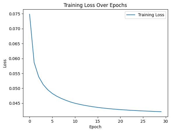
First, here is the training curve with loss for the fingerprint autoencoder
An example of top-10 similarity for a sampled and reconstructed pseudo-fingerprint is shown here
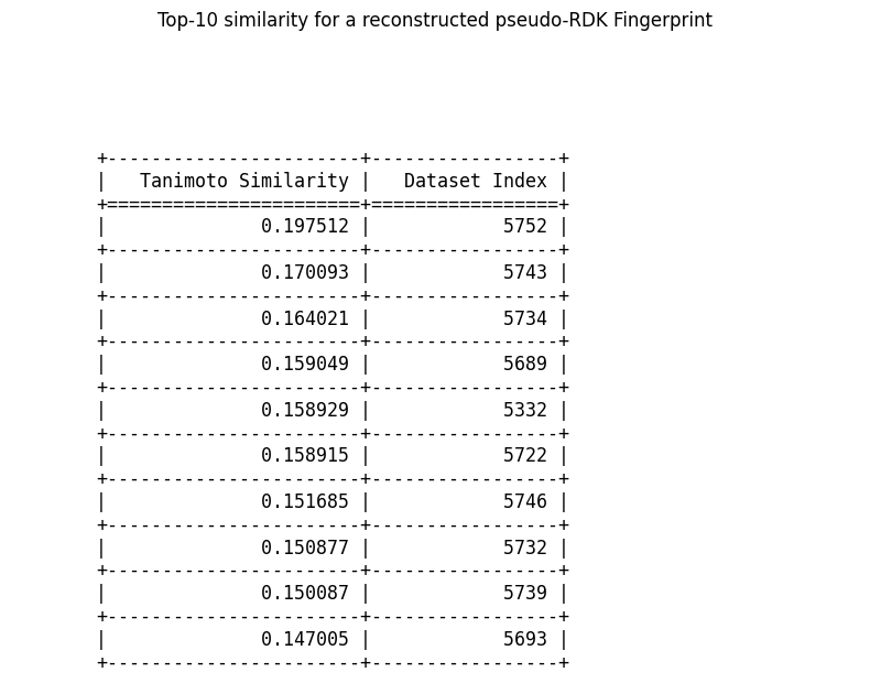
We notice that all the top-10 most similar molecules seem to be near each other, index-wise. This would make sense if the dataset is organized such that similar molecules share close indices. We can confirm this fact by inspecting a heatmap of 10 samples from a consecutive block in the dataset, like so:
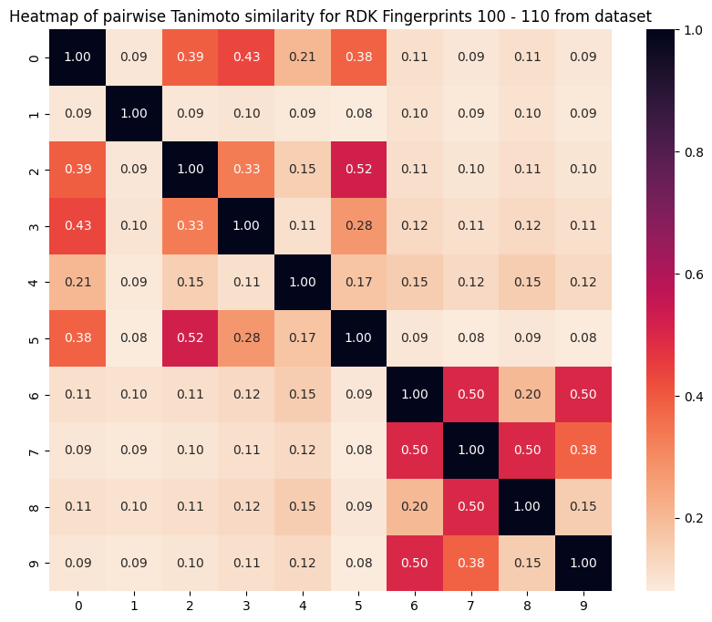
We can see that indeed, closer molecules in the original dataset have higher similarity, so this result is as expected.
Autoencoder Results - Adjacency Matrix
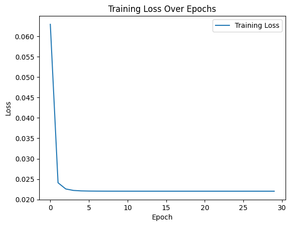
We then inspect the results of the adjacency matrix-based autoencoder training. First, the training curve with loss:
Now, here is a top-10 similarity example for a pseudo-RDK fingerprint from a pseudo-adjacency matrix:
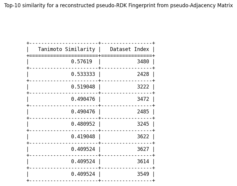
We notice first, that the average similarity is much higher in this case, suggesting that even with the extra step of conversion and the assumptions we make about molecular form, the similarities are higher in this case. The second observation is that the top-10 similar indices are spread out farther than they were in the previous case, suggesting that the adjacency matrix to RDK fingerprint conversion moves around the similar molecules.
Finally, we include some photos of molecules generated in this process (we were unable to generate photos in the RDK fingerprint trained autoencoder, because we require an adjacency matrix to draw the molecules, and it is not straightforward to go from fingerprint to matrix):
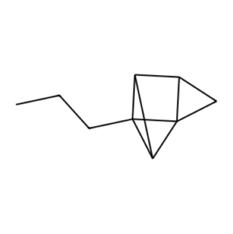
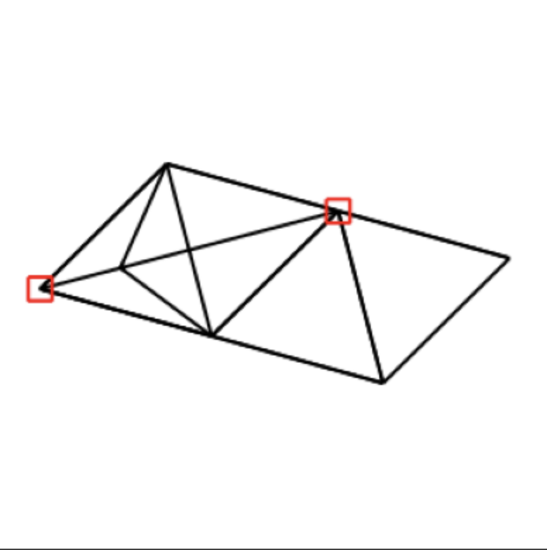
In the photo above, we can see the lefthand side tail as a recognizable part of an organic molecule, suggesting success with some types of bonds. In the photo below, we see that the autoencoder has learnt some additional aspects beyond basic single bonds (one of the validation images we show further below includes a similar red ring).
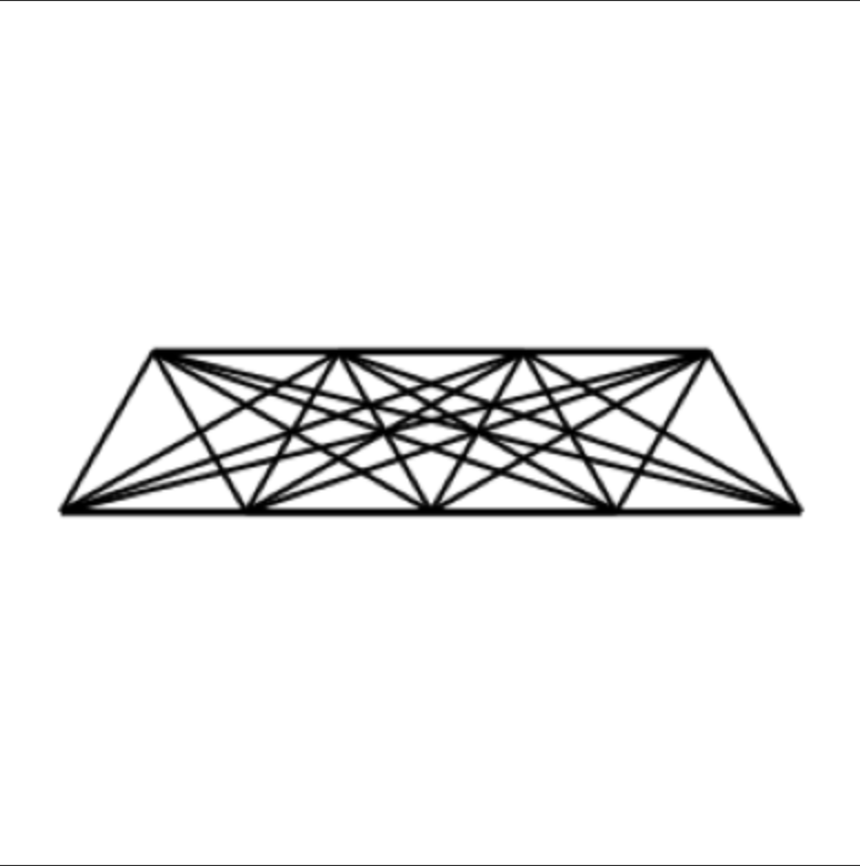
Finally, the photo below while the least small-molecule-like in appearance, is interesting because it appeared many times in samples of 100 images (around 20 times) despite the latent space adjacency matrices being distinct. This could perhaps have to do with the process of converting from an adjacency matrix of reals (the result of latent space sampling) to an adjacency matrix of 1/0s, which we accomplish with median thresholding.
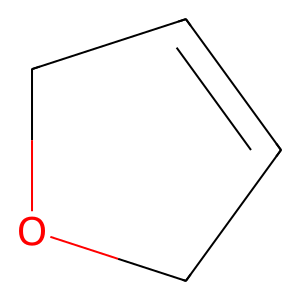
For reference, a sample image from the “validation” true small-molecule dataset is shown below:
Diffusion Model
More recently, the use of diffusion models as an approach for generative modeling has become more common; as described in the introduction, denoising diffusion models operate by iteratively adding noise in a Markov manner to samples, learning the correspondence between inputs and the resultant noise, and then reverse-sampling from random noise to generate a new datapoint.
In the past, as seen in the E3 paper, diffusion models have been applied to 3D adjacency matrices. In this case, we adapted an image-based diffusion model to noise and then de-noise data on adjacency matrices by using 2D adjacency matrices instead.
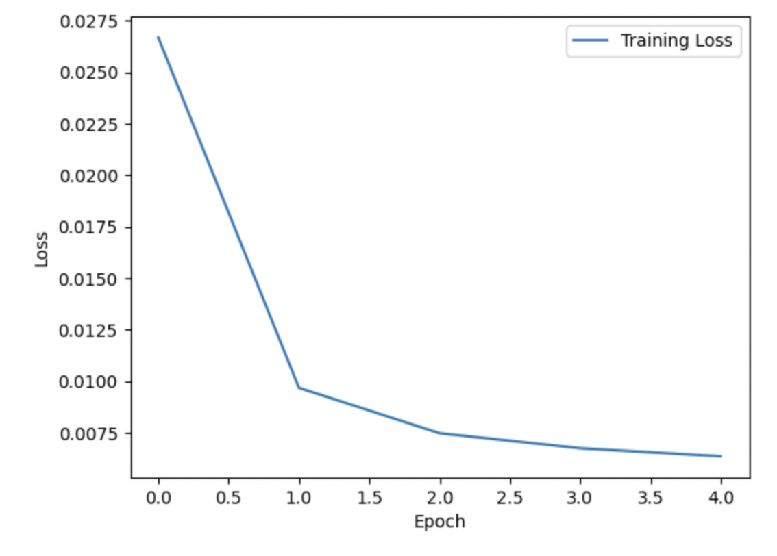
The following plots provide information about the training of the diffusion model on adjacency matrices. First, is a plot of the loss over 5 training epochs at LR 0.001; this model was trained on approximately 90K training samples, so the loss was quite low even after the first epoch:
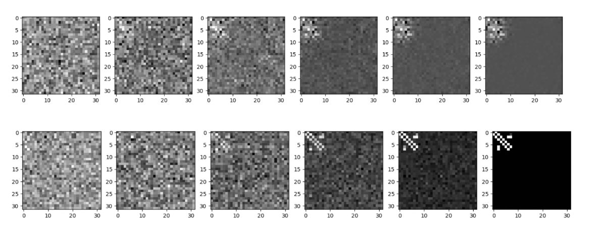
The efficacy of diffusion models as a means of generating novel adjacency matrices is evident from the following visualizations of our results. First, here are two runs of the denoising process for the diffusion model, first on an extremely limited set of approximately 1000 matrices, and then on the entire 90K dataset. As seen, even with very few inputs, it was possible to identify the emergence of a ‘bright spot’ in the top left, which represents the actual adjacency matrix (which was later encoded into actual matrices).
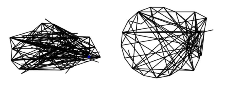
In converting these adjacency matrices into actual molecule images, we aimed to visualize the backbones of these molecules (which is most informative as to the overall structure), so instead of focusing on determining atomic identity, we instead labelled all of them as carbons and proceeded.
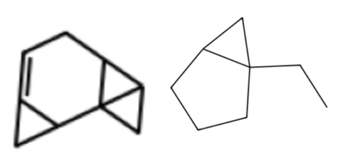
Notably, in comparison to the molecules created by the autoencoder, these contain more of the structures which are characteristics of organic molecules, such as 5 and 6 carbon rings with molecules (potentially side chains of length >1) coming off. Indeed, it is possible to observe the progressively increased ordering of the adjacency matrices over times (as they become closer and closer to actual molecules), going from extremely disordered to closer and closer to something meaningful.
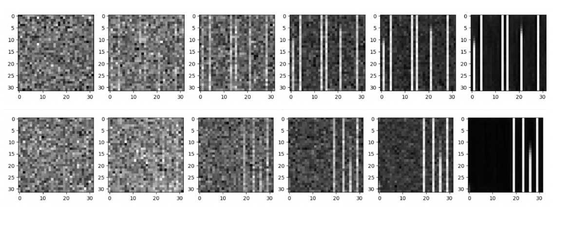
The application of diffusion models to the RDKFingerprints is shown here: for two separate runs, they look like this. Notably, in order to use an image classification network for RDKFingerprints, the fingerprints were stacked into an image which looks like a series of stripes. As evident, the diffusion model was able to produce such striped images, and their simplicity is a good indication that these are indeed good learnings of information about the filtered subset.
Conclusion
In this post, we used two different generative models and tested out two different encodings for information about molecular structure. In general, both models were able to learn and reproduce information about the chosen subset, but in general, the diffusion model was better at accurately reproducing molecules with ‘believable’ structures; as evident from the figures above, although the autoencoder did learn and create relatively sparse adjacency matrices, they lacked the hallmarks of small organic molecules (like rings structures). Further, although it was more difficult to discern quantitative information about the ‘accuracy’ of adjacency matrices, since they depend on larger structures than the RDKfingerprints, it was much easier to map adjacency matrices to actual (visualizable) structures. On the whole, the diffusion model was better at actually creating canonical molecular structures. Further, models trained on adjacency matrices, when converted post-generation to RDKFingerprints had higher accuracy, and adjacency matrices were generally easier to conceptualize, so we have preference for this data encoding.