Contrastive Representation Learning for Dynamical Systems

A deep learning method of learning system underlying parameters from observed trajectories

Introduction

Dynamical System

Dynamical systems form the foundation for understanding intricate phenomena in both scientific research and engineering applications. These systems are defined by their state (denoted as $X$) at any given time and a set of equations (e.g., $v = \frac{dX}{dt} = f_t(X, \theta)$) that describe the evolution of these states over time ($t$), all driven by underlying parameters $\theta$. Some real-world examples of dynamical systems include:

Climate Systems: Involves states like temperature, pressure, and wind velocity, with parameters such as solar radiation and greenhouse gas concentrations.
Population Dynamics in Ecology: Features states like population sizes, with parameters including birth and death rates, and interaction rates between species.
Economic Models: Focus on states like stock prices and trading volume, influenced by parameters like interest rates and market sentiment.
Control Systems in Engineering: Encompasses states like the position and velocity in robotics or the aircraft’s orientation in flight dynamics, governed by parameters like physical properties and control gains.

The evolution of the system’s state over time can be observed as a time series, where system underlying parameters ($\theta$) governs the system’s behavior. In our project, we would like to determine if it would be feasible to discover the underlying system parameters given the observed trajectory. It would lay the groundwork for both robust predictive modeling and model interpretability analysis for safety-critical systems, such as clinical application and chemical engineering plants.

Spring-Mass System

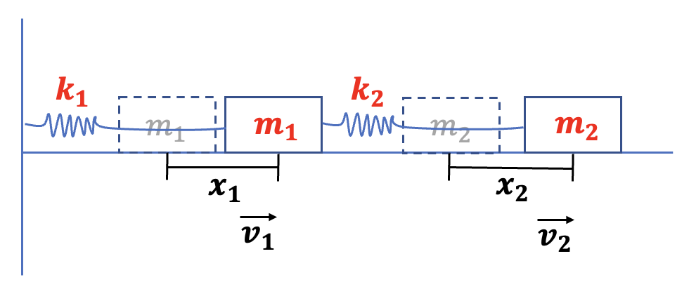
Consider a spring-mass system, a fundamental model in dynamics. In a system comprising two masses, the states include positions $x$ and velocities $v = \frac{dx}{dt}$, which can be derived from the positions. Crucially, it is the underlying parameters, masses $m_1$, $m_2$ and spring constants $k_1$, $k_2$, that dictate the trajectories of $x$.

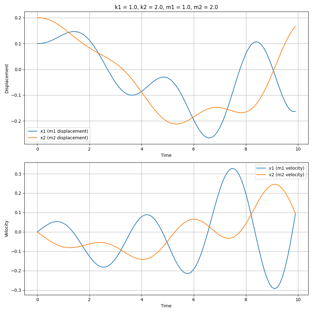
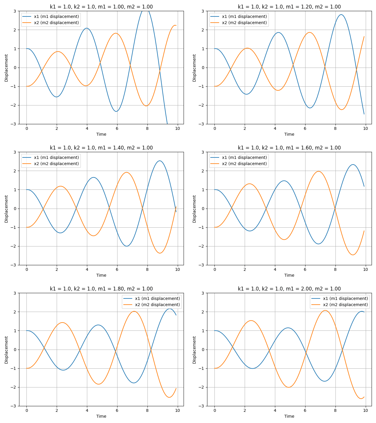
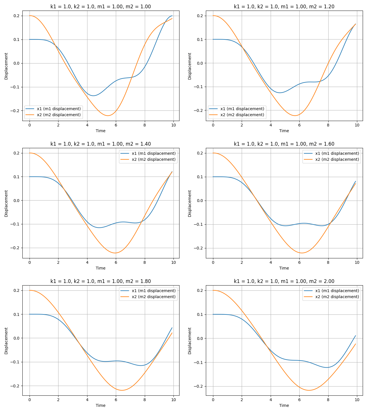
Figure 1: A spring-mass system, classical dynamical system to illustrate project idea

Figure 2: Spring mass system trajectory at ($k_1$, $k_2$, $m_1$, $m_2$) = (1.0, 2.0, 1.0, 2.0)

Different system parameters, such as mass or spring constant, result in different oscillatory and long-term behavior behaviors of the system. Below is a gif demonstrating the effect of changing parameters on the system’s trajectory; this visualization illustrates how different underlying parameter values lead to distinct dynamical behaviors.

Figure 3: system dynamic at varying $m_1$, while keeping $k_1$, $k_2$ and $m_2$ constant.

Figure 4: system dynamics at varying $m_2$, while keeping $k_1$, $k_2$, and $m_1$ constant.

Dataset Collection / Generation

We create a simulator for the above dynamical system to generate data based on parameters like masses $m$ and spring constants $k$. The parameters are systematically varied to generate a diverse and challenging dataset. More concretely, the dataset can be represented by a tensor of shape $(N_{param}, N_{traj}, T, d)$, where:

$N_{param}$ is the number of parameter sets. Each set of parameters would lead to different system dynamics and trajectories.
$N_{traj}$ is the number of trajectories generated for each parameter set. Within the same set of parameters, different initial conditions and noise level would lead to different trajectories.
$T$ is the number of steps in a trajectory. $T$ is dependent on 2 factors - time span in the simulation, and the time step (i.e., $dt$). Note that our system/model formulation allows $T$ to be different for different trajectories, offering more flexibility.
$d$ is the number of states. In the above example, $d = 4$, representing $(x_1, x_2, v_1, v_2)$.

Time-series data analysis is a crucial component in a wide array of scientific and industrial domains, ranging from dynamical systems and weather forecasting to stock market prediction. These applications often involve underlying parameters that are complex and not immediately observable from the data. Traditional time-series methodologies primarily emphasize prediction, which can result in models that operate as “black-boxes” with limited interpretability .

To address this limitation, the representation learning landscape in time-series analysis has expanded recent years, with a focus on unsupervised and semi-supervised methods. Fortuin et al. developed GP-VAEs, combining Gaussian processes with VAEs to handle noisy and irregularly sampled time-series data. This model addresses variabilities in time-series data, offering robust feature extraction. Franceschi et al. explored self-supervised learning frameworks for time-series, demonstrating how leveraging temporal coherence can improve feature representation without reliance on labeled data.

Building on these advancements, recent studies like those by Eldele et al. have explored the application of contrastive learning for enhancing time-series representation. Their approach creates representations by contrasting segments of time-series, thereby learning features that distinguish different temporal patterns. This method has shown promise in enhancing classification and forecasting tasks.

However, there remains an unexplored potential in utilizing contrastive learning for learning the underlying parameters governing these systems. In this project, we aim to bridge this gap by applying the principles of contrastive learning to the specific challenge of identifying and understanding these hidden parameters within dynamical systems. By leveraging contrastive learning, we aim to move beyond mere prediction and delve into a deeper understanding of these parameters, thus enhancing the interpretability of time-series models, particularly applicable in safety-critical systems.

Methodology

Contrastive Learning

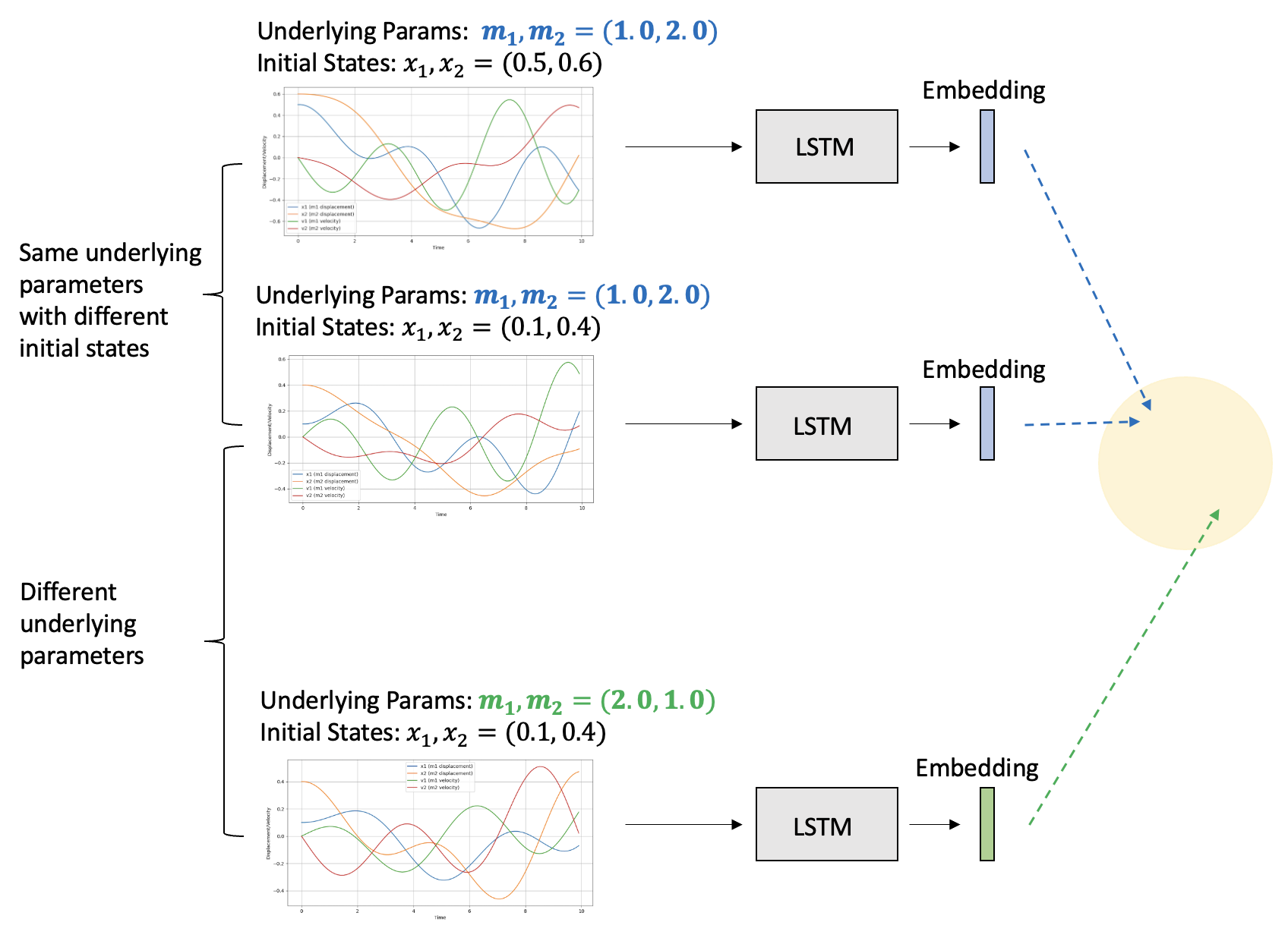
Contrastive learning is a self-supervised learning technique prevalent in fields such as computer vision (CV) and natural language processing (NLP). At its core, it involves minimizing the embedding similarity between similar objects (i.e., positive pairs) while distancing dissimilar ones (i.e., negative pairs).

In the context of dynamical systems, where the model does not have direct access to parameter values, contrastive learning is an effective method to infer underlying system parameters. In our case of spring-mass system, a positive pair consists of two trajectories generated using the same set of parameters, whereas a negative pair is two trajectories generated using different set of parameters.

We utilize the following InfoNCE (Information Noise-Contrastive Estimation) loss for training:

\[L_{\text{InfoNCE}} = -\log \frac{e^{f(x)^Tf(x^+)/\tau}}{\sum_{i=0}^{N} e^{f(x)^Tf(x^-_i)/\tau}}\]

$f(x)$ is the generated trajectory embedding.
$\tau$ is a (fixed) temperature hyperparameter, which we set to default 1.
($x$, $x^+$) forms the positive pair (i.e., two trajectories with the same underlying parameters but different initial conditions).
($x$, $x_j^-$) form negative pairs (i.e. two trajectories from different underlying parameter sets).

Model

Trajectories in dynamical systems can be represented by a time-series dataset, which is a type of sequential data. Long Short-Term Memory networks (LSTMs), a variant of Recurrent Neural Networks (RNNs), can be used process sequential data and manage long-term dependencies. A key feature of LSTMs is their use of gates, which regulate the flow of information, allowing the network to maintain pertinent information over extended periods — key characteristics for modeling dynamical systems. These gates include:

Forget Gate: Decides which information from the cell state should be discarded. It uses the current input and the previous hidden state to generate a value between 0 and 1 for each number in the cell state, with 1 indicating “keep this” and 0 indicating “discard this.”
Input Gate: Determines what new information will be added to the cell state. It involves two parts: a sigmoid layer that decides which values will be updated and a tanh layer that creates a vector of new candidate values.
Output Gate: Decides what information from the cell state will be used to generate the output. It takes the current input and the previous hidden state, passes them through a sigmoid layer, and multiplies the output by a tanh of the cell state to decide which parts of the cell state make it to the output.

Figure 5: Diagram of LSTM .

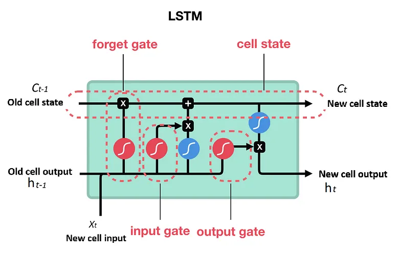
In the context of the contrastive learning framework, the choice of model is a design choice. Essentially, any model capable of converting a trajectory into an embedding, such as a transformer, could be utilized. While transformers have shown remarkable results in CV and NLP, their performance on smaller datasets remains an area less explored. Previous studies in dynamical systems have predominantly employed RNN-based approaches. In this project, we aim to study if LSTM is capable of capturing the dynamics of system through its hidden and cell states.

Training objectives

Trajectories are passed through an LSTM to generate trajectory embeddings, derived from the cell states of the LSTM’s final layer. In our training framework, there are 2 loss functions:

Contrastive objective (InfoNCE loss) is applied on the trajectory embedding. This loss encourages model to create embeddings that meaningfully distinguish between different system dynamics.
Prediction objective (MSE) is applied between the ground truth state (i.e., $X_{t+1}$) and the prediction state (i.e., $\hat{X}_{t+1}$) at the next step. This loss encourages model to use the current state and embedding to predict next step behavior.

Figure 6: Diagram of contrastive representation learning in this project. Trajectories derived from the same parameter set (e.g. top two trajectories in figure) form a positive pair; they map closely in latent space and show invariance to initial states. Trajectories from different parameter sets are distant in latent space, despite identical initial states (e.g. bottom two trajectories).

Evaluation

The objective of the project to estimate the system parameters from observed trajectories. Therefore, the primary metric for our evaluation strategy is the MAE on underlying parameter estimation. This involves applying linear probing to the model’s embeddings against known ground truth parameters on a subset of the training set (i.e., a linear system $X\beta = Y$ is solved, with X representing the trajectory embeddings, and y being the ground truth parameters). Since it is a simple linear transformation of the original features, it has limited capacity to alter feature complexity. Essentially, if a model can perform well under linear probing, it suggests that the learned embeddings themselves are robust and informative with respect to the underlying parameters.

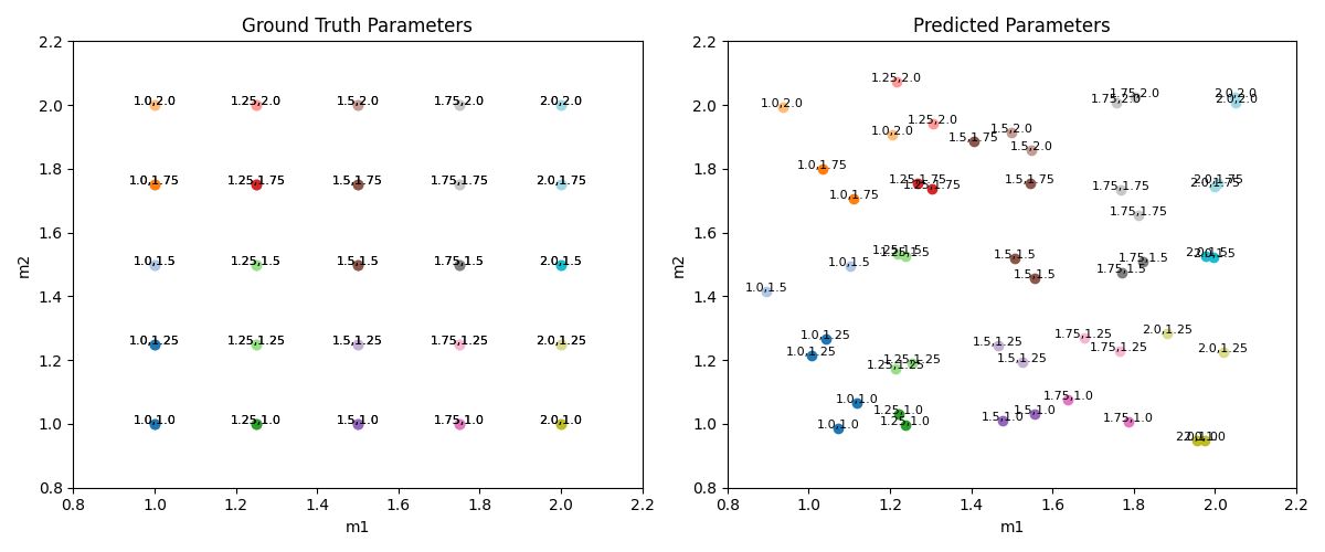
The following plot shows the result of the contrastive learning framework on the validation set. Left subplot corresponds to the ground truth parameter, right subplot corresponds to the predicted parameter using the above contrastive learning framework. For a focused visualization, we only varies 2 parameter (i.e., $m_1$, $m_2$). Each point in the plot is annotated with its corresponding parameter values. For each parameter set, we evaluate on 2 trajectories with different initial conditions.

On the right plot, we observe similar data points are grouped together in the parameter space, indicating that the model is capable of clustering trajectories generated from the same parameter set together. Comparing the left and right plots, we observe the model is capable to predicting parameters to be close to ground truth parameters. Overall, the MAE for parameter estimation is 0.043, underscoring the model’s precision in parameter prediction.

Figure 7: Result of parameter estimation. Left subplot corresponds to the ground truth parameter, right subplot corresponds to the predicted parameter using the above contrastive learning framework.

Additionally, we would also like the model to be capable of predicting the future trajectories. For this objective, the secondary metric is the MAE on next-step prediction. High value on this metrics would indicate model’s ability to accurately forecast future states, which is a necessary but may not be sufficient step towards a more complex, weekly-supervised parameter inference tasks. The MAE on the validation set is 0.00024, and we will discuss it more in the Experiments section.

Experiments

In the previous section, Figure X above shows the final result. We want to include 2 components in this section: 1) different things we attempted to reach the results in Figure X, and 2) several experiments to study how different factors affect model’s capability of discovering the underlying parameters.

Due to computational and time limitation, the numbers reported in this section are not from the final model, which trained for a much longer time. Instead, we ran numerous experiments and compared performance after 2000 steps, at which point the training loss has roughly plateaued.

Effect of initial conditions

The effect of different initial conditions in dynamical system is analogous to the effect of data augmentation in CV. The challenge is that different initial conditions may affect the trajectories more than the change in parameter.

We initially used the same initial conditions for all set of parameters and led to parameter MAE of 0.01 in the validation set. However, the model doesn’t generalize to other initial conditions; when evaluating the model on the validation set that has different initial condition, MAE increased to 0.31, indicating overfit.

To ensure our model effectively discerns differences in trajectories arising from varying initial conditions, we generate 100 trajectories from each parameter set with random initial conditions, aiming to train the model to be invariant to these initial conditions and capture the essence of the system parameters. With this “data augmentation”, we bridged the gap between training and validation performance to be 0.061 and 0.065 respectively.

Number of prediction steps

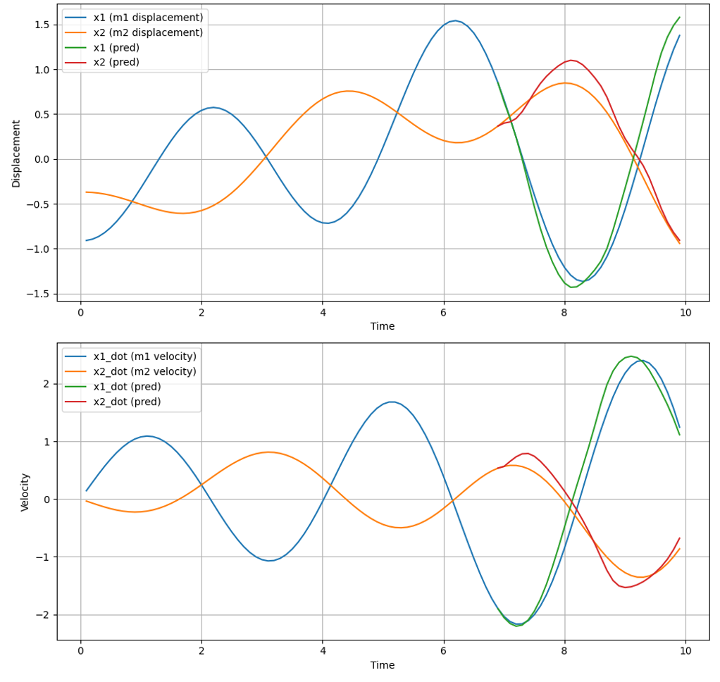
We also considered the limitations of next-step prediction, particularly for high-frequency samples (i.e., small $dt$). A trivial model might simply predict state $X$ at time $t+1$ as $X_t$, and achieve a small loss since $X_{t+1} - X_t$ may be small for small $dt$. To avoid model taking shortcuts, we shift our focus from immediate next-step prediction to forecasting next-k-steps ahead. We also anticipate that accurate longer-horizon predictions would require a deeper understanding of the underlying parameters, potentially leading to improved performance in parameter estimation. This improves the parameter MAE on the validation set from 0.10 to 0.065. The following figure illustrates an results of predicting 30 steps ahead.

Figure 8: Ground truth and predicted trajectory for predicting 30 steps (i.e., 3 seconds).

Decouple state and parameter embedding

In our hypothesis, the latent space of a trajectory encodes dual forms of information: “long-term” information pertaining to system parameters, and “short-term” information reflective of the current state. Traditional approaches applying contrastive learning across the entire latent vector may not optimally capture this duality.

To address this, we propose to decouple the state and parameter embedding space. Concretely, for positive pairs emerging from identical parameters but divergent initial conditions, our approach focuses on computing the InfoNCE loss solely on the segment of the embedding representing the parameter. This is operationalized by limiting contrastive learning to the initial W dimensions of the latent vector, denoted as $z[:W]$. This strategy aims to specialize $z[:W]$ in encoding system parameters, while allowing the remaining part of the vector, $z[W:]$, the flexibility to encapsulate other trajectory aspects, such as initial conditions and inherent noise.

However, the performance didn’t increase across various values of $W$. This stagnation might stem from our use of the LSTM cell state as the latent embedding. Given that the cell state inherently integrates “long-term” information, with “short-term” data predominantly residing in the hidden states, restricting ourselves to $z[:W]$ potentially reduces the representational power of our contrastive learning framework.

Effect of key hyperparameters

We utilized WandB for a hyperparameter sweep to investigate their impact on the model’s performance in next-steps prediction and underlying parameter estimation. Key hyperparameters explored include:

Embedding Size: We observed that increasing the embedding size from 10 to 200 led to a reduction in the InfoNCE loss from 0.862 to 0.007, and the corresponding parameter estimation estimation MAE peaked when embedding size reached 100. This suggests a larger embedding size can increase the capacity to more effectively inferring underlying system parameters. However, maintaining the embedding size at a balanced level is crucial to ensure the model concentrates on the most pivotal aspects of data variation, rather than overfitting to minor system details.
Number of LSTM Layers: Increasing the number of LSTM layers improved both next-step prediction and parameter estimation. Notably, with more LSTM layers, a smaller embedding size became sufficient for achieving desirable outcomes in both prediction and parameter inference. This implies a deeper LSTM architecture can capture more complex pattern in the data.
Prediction Horizon (Predict Ahead): We observe a modest improvement in performance on parameter estimation MAE (i.e., 0.04) as the prediction horizon increases. This improvement, while positive, was less pronounced than anticipated. In our model, contrastive learning serves as the primary mechanism for learning about system parameters, with next-k-step prediction intended to supplement this learning process. Theoretically, as the prediction horizon (k) increases, the complexity of the next-k-step prediction task escalates. This demands more focus from the model, potentially at the expense of its capacity for contrastive learning. Consequently, the variable k emerges as a hyperparameter to strike an optimal balance between two competing objectives: facilitating overall learning (where a larger k is advantageous), and maintaining a focus on contrastive learning (where a smaller k is beneficial).

Noise level in data generation

In real-world applications, models often lack direct access to state values due to the inherent stochasticity of systems or observation noise. In high-precision engineering applications, this noise is typically constrained to below 1%. However, in less precise scenarios, the noise in observed data can reach levels as high as 20%. It’s important to note that these errors are not merely observational errors, which can be assumed to be independent and identically distributed (i.i.d). Rather, these errors are intertwined with the state itself and can propagate over time, affecting subsequent observations. The figure below illustrates how noise can significantly alter trajectories. For instance, at a 20% noise level, the state variable $x_1$ markedly diverges from its intended path around the 8-second mar

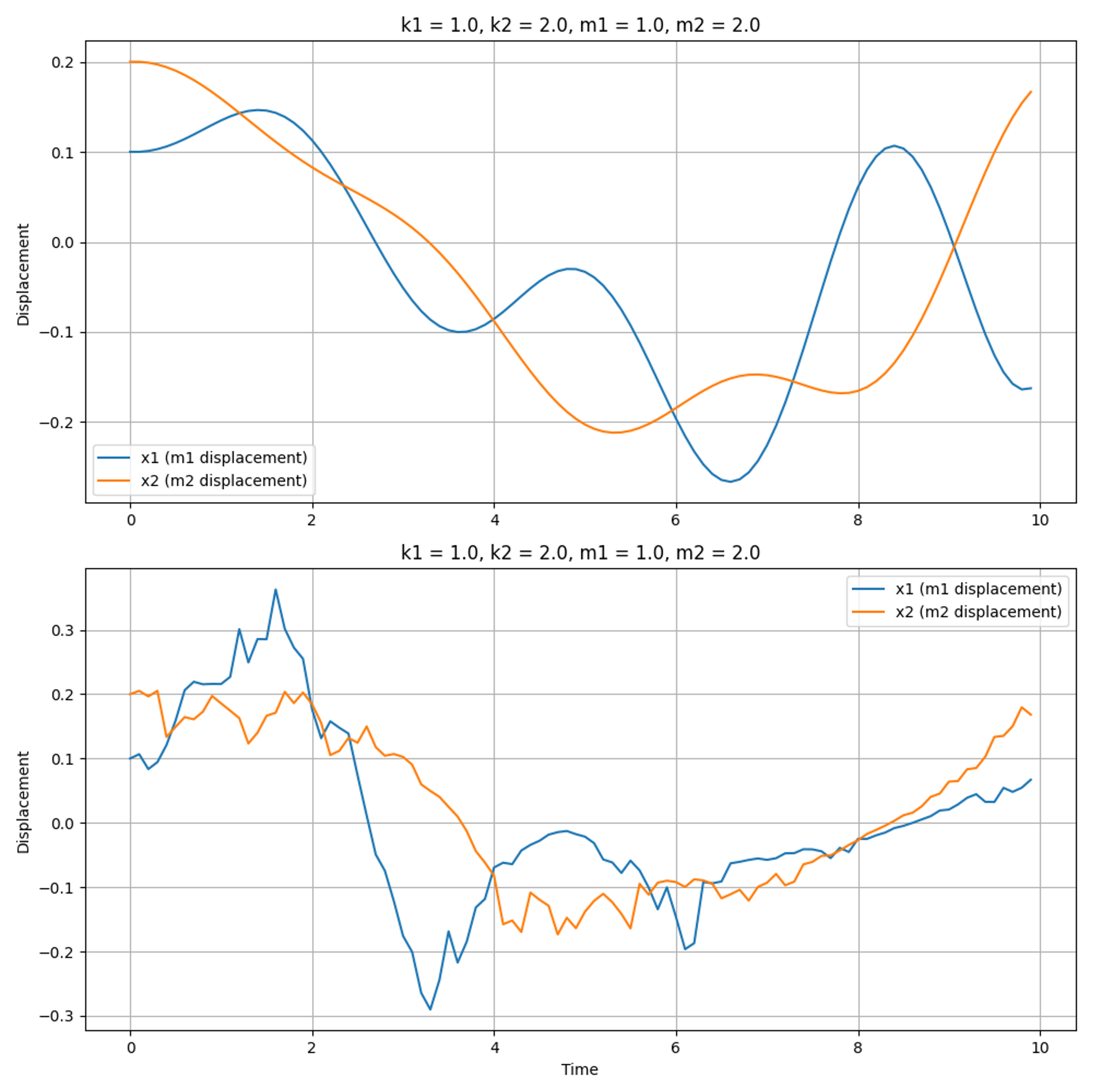
Figure 9: Comparison of state trajectories with no noise (top subplot) and 20% noise (bottom subplot).

The following section evaluates the model’s performance using noisy observed data. During trajectory generation, we introduce random noise according to the formula $X_{obs} = X_{true} (1 + \alpha \mathit{N}(0, 1))$ where $\alpha$ is the noise-to-signal ratio. We studied the model’s performance across various noise levels, ranging from $\alpha = 0.0$ to $\alpha = 0.2$, and the results are plotting in the following figure.

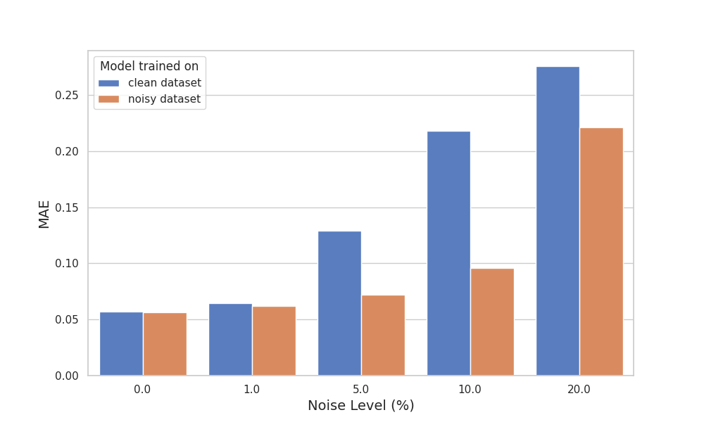
Figure 10: Model performance across different noise levels. The blue bars represent a model trained on a clean dataset, and directly applied to a noisy validation dataset. The orange bars represent a model trained and evaluated on datasets with equivalent noise levels.

Directly applying a model trained with a clean dataset on a noisy dataset would lead to drastic performance drop as shown in the blue bars. During model deployment, it’s a natural choice to train on a dataset with the same noise amount. This could mitigate the drastic performance drop, especially for low to moderate amount of noise (e.g., $\alpha < 0.1$), as shown in the orange bars. However, when noise amount rises to 20%, training on noisy dataset doesn’t help either due to significant deviation from clean data.

Applying a model trained on a clean dataset to a noisy dataset leads to a significant drop in performance, as indicated by the blue bars. In practical model deployment, it’s common to train the model on a dataset with a comparable level of noise. This approach can substantially mitigate performance degradation, particularly at low to moderate noise levels (e.g., $\alpha < 0.1$), as demonstrated by the orange bars. However, at higher noise levels, such as 20%, training on a noisy dataset proves less effective due to the substantial deviation from the clean data.

Generalizability to unseen parameters

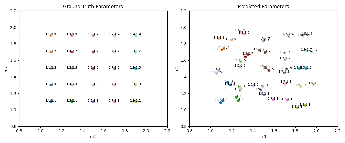
In this section, we delve into the model’s generalizability across unseen parameters. Our investigation comprises experiments on both in-distribution and out-of-distribution system parameters. The results of these experiments are illustrated in the following figures.

For in-distribution analysis, our focus was to assess the model’s proficiency in adapting to system parameters that, while differing from those in the training set, still fall within the same predefined range. This aspect of the study aims to understand how well the model can interpolate within the known parameter space.

Figure 11: Result of parameter estimation to unseen parameters in-distribution.

On the other hand, the out-of-distribution experiments were designed to challenge the model further by introducing system parameters that lie outside the range encountered during training. This approach tests the model’s ability to extrapolate beyond its training confines.

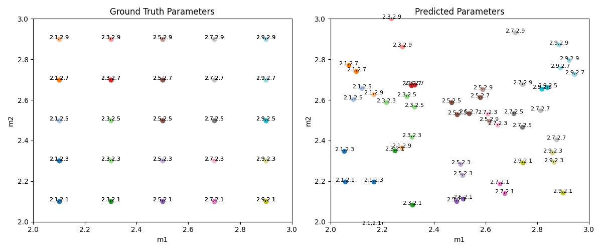
Figure 12: Result of parameter estimation to unseen parameters out-of-distribution.

Remarkably, our model demonstrated a robust ability to generalize across both in-distribution and out-of-distribution parameters. It achieved a Mean Absolute Error (MAE) of 0.032 in the former and 0.082 in the latter scenario. These findings suggest that the model not only learns the underlying patterns within the training data but also retains a significant degree of flexibility to adapt to new, unseen parameter sets.

Another Framework - Generative Modeling

While the previously discussed contrastive learning framework shows promise in inferring underlying parameters through a weakly-supervised learning approach, it relies on prior knowledge about the relationship between trajectories and their corresponding parameter sets. Such information may not always be readily available in practical scenarios. To address this challenge, our research pivots towards employing a generative modeling framework, enabling the learning of system parameters in an unsupervised manner.

We transition from contrastive learning to incorporating a variational autoencoder (VAE) structure. This setup operates without explicit knowledge of parameter sets, compelling the model to decipher the underlying patterns solely from the observed trajectories. The VAE framework consists of three primary components: 1) an encoder LSTM that transforms an observed trajectory into a latent representation, 2) a reparameterization layer that molds this latent representation into a specific distribution, and 3) a decoder LSTM that uses the latent representation and initial conditions to reconstruct the trajectory.

Training focuses on 1) the reconstruction loss between real and a generated trajectories, and 2) Mean Absolute Error (MAE) for next-k-step predictions made by the encoder LSTM. This method is designed to challenge the model’s capability to extract insights about the system’s dynamics independently, without relying on any prior information about the trajectories. The framework thus becomes a critical platform for testing the model’s ability to autonomously learn the system’s underlying parameters, requiring an advanced level of unsupervised learning.

The evaluation metrics for this second framework are aligned with the first, utilizing MAE to assess both the underlying parameter estimation and the next k-step prediction accuracy of the encoder LSTM. A key addition in this framework is the MAE on Reconstruction Loss.This metric is used to gauge the model’s ability to accurately reconstruct input sequences, thereby reflecting its understanding of the data’s fundamental structure. A lower reconstruction loss implies that the model has effectively internalized the essential characteristics of the data distribution. Our expectation is that this deeper grasp of data structure will enable the model to infer underlying system parameters independently, without prior exposure to specific parameter set information.

Experiments - Generative Modeling

Autoencoder v.s. Variational Autoencoder

In addition to exploring the Variational Autoencoder (VAE) framework, we also experimented with a traditional autoencoder setup. This variant mirrors the architecture of the VAE but excludes the computation of the mean ($\mu$) and log variance ($\log \sigma^2$), thereby omitting the variational element. This modification streamlines the model, narrowing its focus to purely reconstructing input data from its latent representations.

Our findings reveal that the autoencoder configuration surpassed the VAE in both parameter estimation and reconstruction. For parameter estimation MAE, autoencoder and VAE achieved 0.12 and 0.23 respectively. For reconstruction MAE, autoencoder and VAE achieved 0.02 and 0.49 respectively. This performance disparity can be attributed to the inherent constraints of each model. The autoencoder is primarily limited by the dimensionality of the embedding in its latent space. In contrast, the VAE faces an additional constraint due to its need to model the distribution within the latent space.

These results suggest that the variational component, a defining feature of VAEs and instrumental in modeling data distributions, might not be essential for capturing the dynamics specific to our system. By removing the variational aspect, the autoencoder model is enabled to concentrate more effectively on capturing the most salient features for reconstruction and parameter inference. This simpler approach avoids the additional complexity of encoding the data distribution in the latent space, potentially leading to more efficient and targeted learning relevant to our system’s dynamics.

Beyond Reconstruction: Evaluating Future Prediction Capabilities

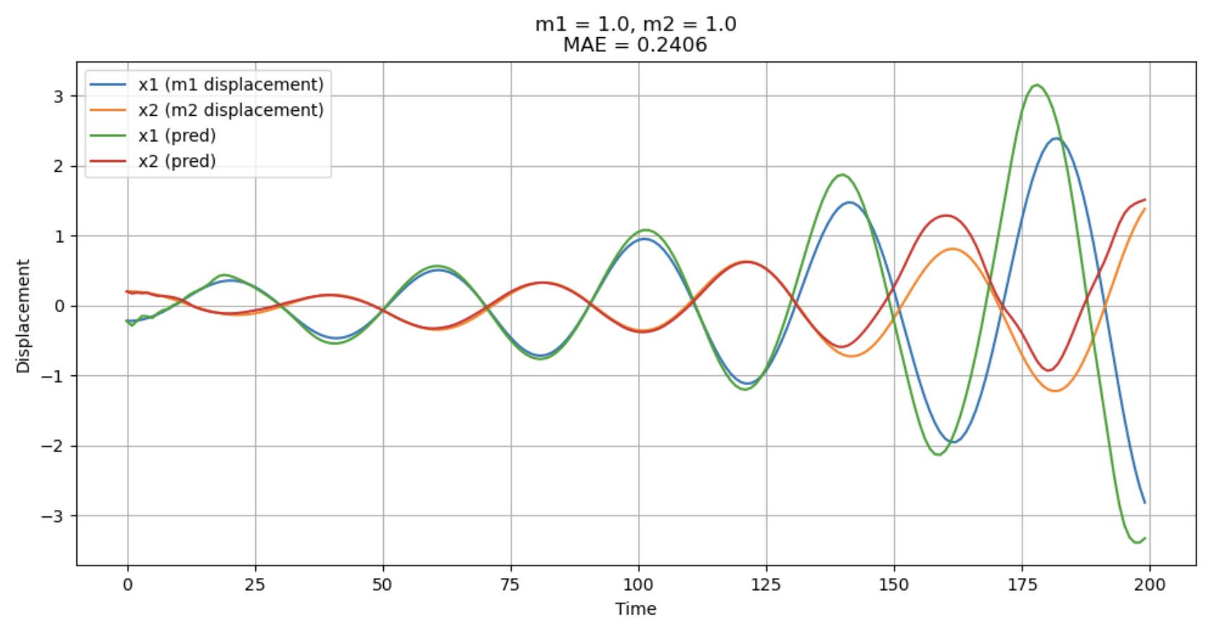
To evaluate our AE model’s generalizability and future prediction capabilities, we expanded its function beyond reconstruction to include forecasting additional steps. The figure presented here compares the ground truth states $x_1$ and $x_2$ (displacements for $m_1$ and $m_2$) against the model’s outputs for both reconstruction and prediction. The model processes input trajectories of 100 time steps and generates outputs for 199 steps, with the initial 99 steps dedicated to reconstruction and the subsequent 100 steps for prediction (unseen by the model during training). The results illustrate effective reconstruction performance but relatively weaker predictive accuracy.

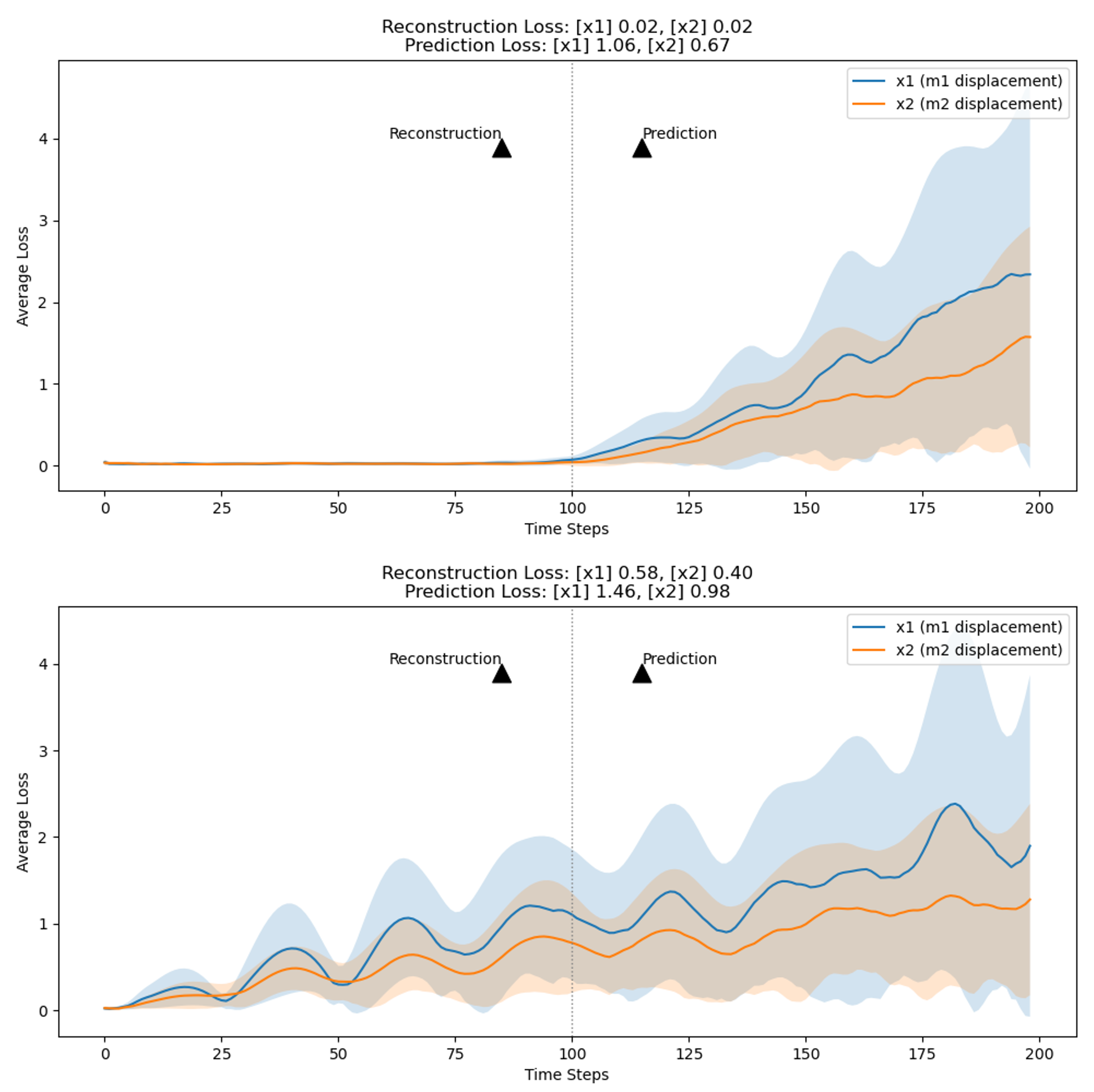
Figure 13: Reconstruction and further prediction of unseen states.

Given that our autoencoder (AE) framework surpasses the Variational Autoencoder (VAE) in reconstruction and parameter estimation, we speculated whether VAE’s variational component might enhance future predictions. Therefore, we compared the reconstruction and prediction losses between the AE and VAE frameworks.

The corresponding figure, presenting the mean and standard deviation of these losses, reveals that in both frameworks, reconstruction losses and their variability are substantially lower than prediction losses. This trend highlights the ongoing difficulty in achieving precise future predictions within our model configurations.

Furthermore, the AE framework demonstrated superior performance over the VAE in both reconstruction and future step prediction. This outcome suggests that the VAE’s variational component does not necessarily contribute to improved future predictions. Echoing our earlier findings on parameter estimation and reconstruction, the variational aspect might not be pivotal for capturing the dynamics specific to our system. Instead, it could introduce additional complexity by encoding the data distribution in the latent space, which appears to be less relevant for reconstruction and future step prediction tasks.

Figure 14: Results of reconstruction loss (first 99 steps) and future prediction loss (last 100 steps) for autoencoder (top subplot) and VAE (bottom subplot).

Effect of Latent Variables on Generated Trajectories

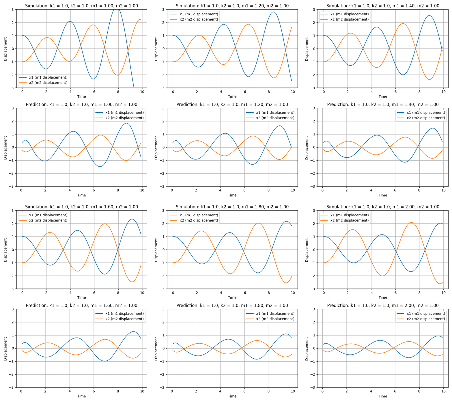
In this section, our objective is to glean insights into the latent variables by manipulating them and observing the resultant changes in the generated trajectories. Given that the embedding dimension (i.e., |z|) exceeds the dimension of the parameters (i.e., |$\theta$|), we initially establish a linear mapping from from $z$ to $\theta$. The following gif demonstrates how the trajectory evolves in response to alterations in the variable $m_1$. The upper part of the gif represents the simulation, while the lower part reflects the output from the decoder of our autoencoder.

A notable observation is that, as m1 undergoes modifications, the predicted trajectories adeptly resemble the period of the simulation trajectories. However, a discrepancy arises in their magnitude, with the predicted trajectories exhibiting a notably smaller scale compared to the ground truth trajectories. This pattern suggests that while the embedding successfully captures certain characteristics of the trajectories, it does not fully encapsulate all their properties.

We hypothesize that enhancing the complexity of the encoder/decoder architecture (e.g., larger number of layers of LSTM layers) might facilitate a more comprehensive capture of trajectory attributes. However, our experimental scope is currently constrained by limitations in CUDA memory, particularly due to the decoder’s requirement to process 99 time steps. This constraint hinders our ability to experiment with architectures involving a greater number of layers, which might otherwise allow for a richer representation and understanding of the trajectory data.

Figure 15: Effect of latent variables on generated trajectories.

Conclusion and Future Works

In contrast to current machine learning literature that predominantly focuses on predicting future states of dynamical systems, our work is geared towards uncovering the underlying system parameters from observed trajectories. Our key contributions include:

Implementing two frameworks: an autoregressive LSTM with contrastive learning, and a variational autoencoder architecture. While contrastive learning yields superior parameter estimation, the autoencoder enables unsupervised learning without relying on prior knowledge.
Demonstrating our model’s generalizability to both in-distribution and out-of-distribution unseen parameters, and its effective performance with noisy datasets, sustaining a noise-to-signal ratio of up to 10%.
Conducting thorough experiments to explore the impact of various factors like initial conditions, prediction horizons, and the interplay between state and parameters embeddings. We also examined the influence of latent variables on trajectory generation and the model’s predictive capabilities beyond the confines of the training set.

The ability to accurately estimate underlying system parameters significantly enhances model interpretability, which is crucial in scientific and engineering applications where decision-making stakes are high. We hope our findings will help researchers and students interested in interpretable machine learning for dynamical systems.

While this project did extensive analysis on a spring-mass system, future work may extend this analysis to a broader range of dynamical systems. Moreover, future work can integrate the strengths of both frameworks to incorporate contrastive learning within an unsupervised context, possibly through data augmentation strategies. Further advancements could also focus on refining the impact of latent variables on trajectory generation. Such progress is expected to bolster trust in AI solutions and facilitate their integration into essential decision-making frameworks across various domains.

Here’s the link to our Github Repo: https://github.com/martinzwm/meta_param_est