VIVformer

A deep transformer framework trained on real experimental and synthetic gen-AI data for forecasting non-stationary time-series. Applications and insights drawn from vortex induced vibrations data collected at the MIT Towing Tank.

Introduction & Motivation

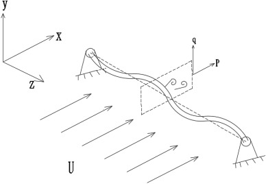
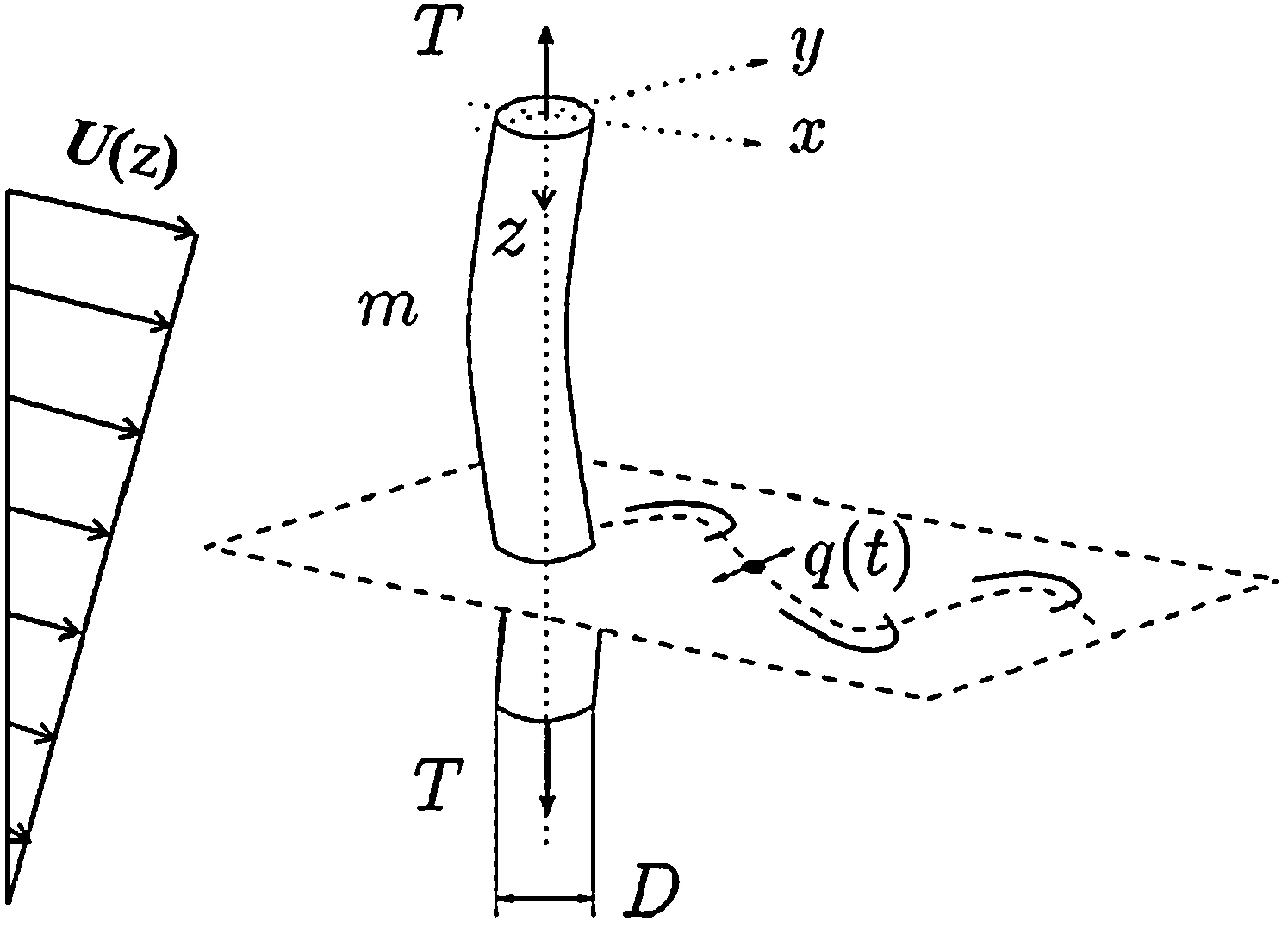
Vortex induced vibrations (VIV) are vibrations that affect bluff bodies in the presence of currents. VIV are driven by the periodic formation and shedding of vortices in the bodies’ wakes which create an alternating pressure variation causing persistent vibrations . The vibration amplitude in VIV is typically moderate, not exceeding about one to two body diameters . For flexible bodies, VIV are not uniform along the body’s length (usally refered to as the span) but rather different points along the span vibrate with different amplitudes and phases.

Schematic diagrams of vortex induced vibrations of flexible bodies.

Observations of vortex induced vibrations (VIV) date back to antiquity, when the Aeolian tones, sounds created by pressure fluctuations induced by winds passing over taut strings were recognized. The first sketches of vortices date back to Leonardo da Vinci in the early 16th century. Today, VIV have become a problem of interest to both theoreticians, due to the complex underlying mechanisms involved, and engineers, due to the practical significance of mitigating the fatigue damage VIV can cause to offshore structures and equipment such as marine risers and offshore wind turbines. In order to gain some intuition, the reader can refer to the video of a flexible body undergoing VIV in section “Data Description” (below).

The underlying driving mechanism of VIV is vortex formation; specifically, the periodic shedding of vortices formed in the wake behind bluff bodies placed within cross-currents . The vortex shedding frequency in rigid bodies is known as the Strouhal frequency. For flexibly mounted or flexible bodies, the vortex formation frequency can be entrained away from the Strouhal frequency and coincides with the frequency of vibration in a phenomenon known as lock-in . This occurs across a wide range of oscillating frequencies resembling a nonlinear resonance . Given that flexible body VIV are not span-wise uniform as the flexible body undergoes a spatially traveling and/or standing wave response from the forcing excerted by the fluid , the observed motions are nonstationary, unsteady, and can transition to different responses even for seemingly unchanged experimental conditions.

VIV of flexible bodies are usually modelled by leveraging the modal decomposition technique (i.e. using a Fourier expansion of sinusoidal mode shapes with time varying coefficients), similar to the approach introduced for modelling vibrating shafts and beams . Recently, Kharazmi et al. (2021) attempted to learn the mode shapes and time varying coefficients using LSTM networks in modal space (LSTM-Modnet); Mentzelopoulos et al. (2023) proposed learning a sparse-mode set of sinusoidal modes along with the corresponding time-varying coefficients. Both frameworks suffer from the inability to robustly forecast future motions.

Although leveraging transformers to expand the horizon of predictions of time series is a very active field of research , transformers have not yet been used to predict VIV of flexible bodies, which are physical non-stationary time-series, to the best of the author’s knowledge. In addition, only limited work has been performed in generating physical data using generative models and there are no identifiable applications to VIV in the literature. Mostly appications of machine learning for VIV include solving physical equations using physics-informed neural networks (PINNs) and learning hydrodynamic coefficients or other relevant quantities in order to predict the motions on average rather than instantaneously .

In this work, an attempt will be made to develop a transformer network architecture to predict the VIV of a flexible body both instantaneously and on average. The transformer will be trained and tested using data collected at the MIT Towing Tank by the author. In addition, in order to make the most of the available data, a variational autoencoder (VAE) will be trained to generate more VIV samples which will then be used to train the transformer. In doing so, the capability of VAEs to create physical data which retain information of the underlying physical processes will also be examined. The rest of the blog will be organized as follows: 1. using generative-AI, specifically variational autoencoders, in order to generate physical VIV data 2. using transformers to model and forecast nonstationary flexible body VIV.

Data Description

All data used for this study were collected during experiments conducted by the author at the MIT Towing Tank, a facility consisting of a 35m x 2.5m x 1.2m water tank equipped with a towing carriage capable of reaching speeds exceeding 2 m/s as well as a flow visualization window. In this and the following sections the terms model, riser, flexible body, and flexible cylinder will be used interchangeably to refer to the flexible cylinder model used during experiments.

The figure below illustrates the experimental setup schematically. A solid aluminum frame was used to support the flexible cylinder; the riser model was placed vertically at the center of the structure. An ATI 6 degree of freedom force sensor was attached to the top end of the riser to measure its tension. Two GoPro Hero 11 cameras were attached to the supporting frame facing perpendicular directions to capture videos of the riser’s motion in the cross-flow and in-line directions, respectively.

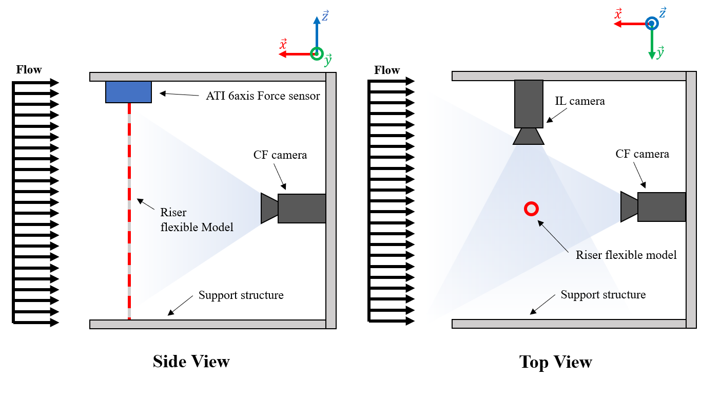
Schematic of experimental setup. A riser model was placed at the center of a supporting frame which was towed resulting in a uniform incoming flow profile on the model.

The riser model was constructed out of urethane rubber infused with tungsten powder. Specifically, Smooth-On PMC-724 urethane rubber was mixed with powdered tungsten to increase the model’s density and achieve a mass-ratio $m^* = \frac{\rho_{model}}{\rho_{H_2O}} = 3$. The mixture was poured into a right cylindrical mold with a fishing line placed along its centerline to provide tension. The model’s length was 890 mm with a 5 mm diameter. The length-to-diameter ratio of the model riser was L/D = 178. Equidistant markers were spray-painted red on the riser model resembling a zebra-patterning to enable motion tracking using cameras. Three underwater light fixtures were used to enhance visibility underwater. The model’s ends were clamped on the supporting frame and the model was separated from the frame by a distance much greater than the body’s diameter $O( > 10D)$.

The flexible cylinder was towed at 0.7 m/s resulting in a uniform incoming flow profile along the x direction, as shown in the schematic above. Recordings of the motions were captured at a resolution of 1080p (1920x1080 pixels) and 120 fps. The Reynolds number was $ Re \approx 3,500$. A visualization of the vibration is shown below (this is a gif of the actual vibration recording downsampled in time).

Sample video recording of the cross-flow vibration of the flexible body (top) and tracking result of the motion (bottom).

Reconstruction of the motion was done using a machine vision framework leveraging Kalman filtering for multi-object tracking; for more information one may refer to Mentzelopoulos et al. (2024) . The high level process is shown below.

Pipeline for motion reconstruction. Red markers on the body were tracked across the video frames to obtain their motion.

A total of 36 locations along the span were marked red on the fexible body and their positions were tracked. The endpoints were fixed on the supporting frame and thus their displacement was zero.

Vibration Data as Images

The displacement of the vibrating body was recorded at 36 uniformly spaced locations along the body’s span and the video recordings were sampled at 120 fps. One may store the vibration data as 2D arrays of $N_{time}$ x $N_{sensor}$, where each row corresponds to a different time of the vibrating body’s displacement at $N_{sensor}$ locations.

Visualization of experimental data. The x-axis corresponds to sensor number (i.e. body location) and the y-axis corresponds to time step (i.e. $\Delta t = 1/fps = 1/120 \ sec$). The displacement normalized by the body's diameter is highlighted on the plane. On the left we visualize the vibration data stored in 2D arrays. On the right, we plot the interpolated values which make more intuitive sense as visualized flexible body vibrations (travelling wave response with peaks travelling to the right from location 0 to location 36). Lines parallel to the x-axis are "snapshots" of the flexible body vibrting in the direction perpendicular to the paper/screen (i.e. "in and out of the page").

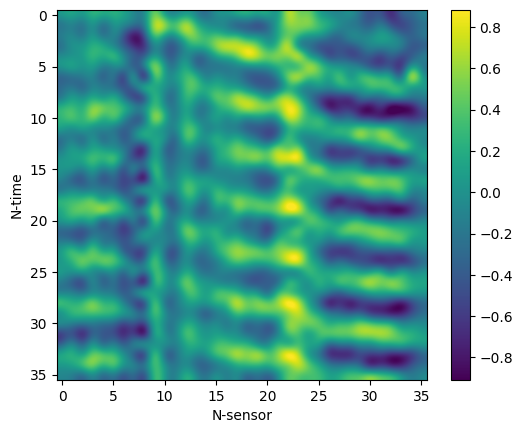
The stored vibration data are illustrated above and can easily be visualized and treated like single channel images! If necessary, scaling pixel values invertibly to an interval of choice, like [0,1] or [0, 255] requires just a few operations leveraging the maximum and minimum values of the data. In the images shown above, each row corresponds to a different time of the recorded vibration at all sampled locations. The time difference between consecutive time steps is $\Delta t = 1/fps = 1/120 \ sec$. The 36 “sensor locations” correspond to the uniformly spaced markers on the body (excluding the two endpoints) and thus they span approximately the full body length. Plotting the interpolated values of the array yileds a more intuitive interpretation of the vibrations. In the data shown above, a travelling wave (crests travelling) from location 0 to location 35 can be identified. For convenience, the data were stored in a single 4D array of size $N_{batch}$ x $1$ x $N_{time}$ x $N_{sensor} = N_{batch}$ x $1$ x $36$ x $36$, yielding hundreds of square arrays of size 36 x 36 which can be easily visualized and collected in batches for training models.

Gen-AI for Physical Vibration Data using Variational Autoencoders

In this section we focus on generating physical vibration data using generative-AI. We will attempt using a variational autoencoder (VAE) trained on the real experimental data described above to generate syntehtic data of the vibrations. We are interested in understanding whether the generated data preserve physicality and thus whether they can be used to train models and to understand the underlying physical generative process by studying the artificial data.

A VAE is a specific network architecture whose goal is to learn a probabilistic mapping from an input space to a low dimensional latent space and then back to the input space. The network architecture is comprised of an encoder network which maps data from the input space to the latent space and a decoder network which maps data from the latent space back to the input space. A schematic of the VAE used for this work is shown below.

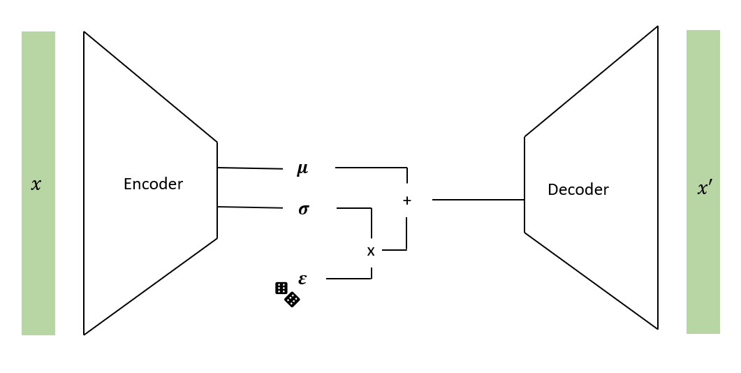
Schematic of the variational autoencoder architecture.

On a high level, the variational autoencoder acts just as a regular autoencoder, with the difference that the training ensures that the distribution of the data in the latent space is regular enough to enable a generative process when sampling from the latent space. That is, the minimized loss ensures that the distribution of the data over the latent dimensions, $q(z \mid x)$, is as close to a standard normal distribution as possible. We choose to assume a Gaussian prior on the latent space for our data since we will need to sample from it when decoding, a task which is nontrivial for arbitrary distributions. The decoder on the other hand will learn the distribution of the decoded variables, $p(x \mid z)$ given their latent representations.

The encoder architecture of choice was the following, accepting an input $x \in R^{36 \times 36}$:

$x \rightarrow Linear (R^{36 \times 36}, R^{64}) \rightarrow ReLU \rightarrow Linear(R^{64}, R^{64}) \rightarrow ReLU \rightarrow x_{embedding}$
$x_{embedding} \rightarrow Linear(R^{64}, R^{5}) \rightarrow ReLU \rightarrow \mu \in R^5$
$x_{embedding} \rightarrow Linear(R^{64}, R^{5}) \rightarrow ReLU \rightarrow \sigma \in R^5$

where $\mu$ and $\sigma$ are the mean and variance of the posterior data distribution in the latent space. The decoder architecture was as follows accepting an input $z \in R^5$:

$z \rightarrow Linear(R^{5}, R^{64}) \rightarrow ReLU \rightarrow Linear(R^{64}, R^{36 \times 36}) \rightarrow ReLU \rightarrow x^\prime$

Training was done by maximizing the evidence lower bound (ELBO) on the experimental data and the outputs of the autoencoder. This is equivalent to minimizing the following loss (negative of ELBO).

$Loss_{ELBO} = - E_{q(z \mid x)} \bigg[ \log p(x\mid z) - D_{KL}(q(z \mid x )\mid \mid q(z)) \bigg]$

where $D_{KL}$ referes to the Kullback-Leibler divergence. Intuitively, maximizing the ELBO or minimizing the above $Loss_{ELBO}$, aims at maximizing the log-likelihood of the data given their representations in the latent space while minimizing the Kullback-Leibler divergence between the learned posterior of the data in the latent space and the prior assumption of a Gaussian distribution in the latent space. For the purposes of training, the data were scaled to be between [0, 1] in order to use binary cross entropy. The VAE was trained using Adam optimizer with a learning rate $lr = 0.01$. A step scheduler was set to decay the step by $\gamma = 1/2$ every 2,000 iterations. The training loss as a function of epoch is shown below.

Training loss ($Loss_{ELBO}$) for the VAE on the input real VIV data.

Having trained the VAE, samples from the standard normal distribution in $R^5$ were drawn, decoded, and rescaled in order to generate synthetic VIV data. Three random samples are included below (top), along with three random samples of real data observed during experiments (bottom).

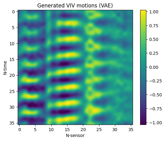
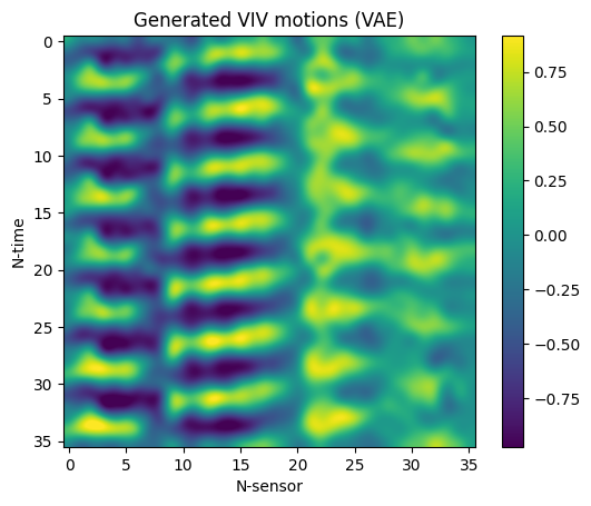
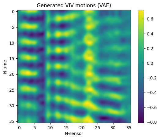
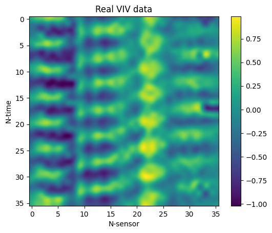
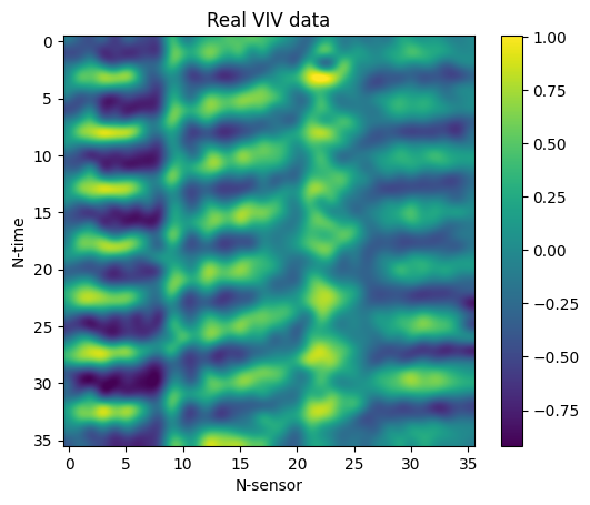
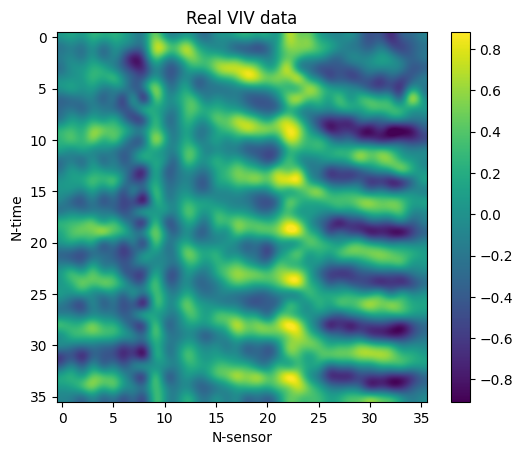
Top row: Generated data using the VAE. Bottom row: Real data recorded from experiments.

Albeit the data generated data are certainly eye-pleasing, their promise begs the question of whether they preserve physicality. In order to address this question, we will examine whether a model trained on synthetic data can be used to predict real experimental data.

VIVformer - A Transformer Architecture for VIV

Tranformer network architectures have been widely used and are considered state of the art tools for various machine-learning tasks, particularly in natural language processing (NLP) and computer vision. The transformer architecture has become a cornerstone in deep learning and its applications span across all fields of engineering and science. In this section we will develop a transformer architecture to model and forecast the VIV of flexible bodies under the excitation of a hydrodynamic force. The transformer architecture used for this purpose is shown below.

VIVformer: A transformer architecture for vortex-induced vibrations.

As shown schematically above, the architecture is comprised by various Residual-Attention modules followed by a final linear layer. The input to the VIVformer is a batch of vibration data as discussed in previous sections “Data Description” and “Visualizing the Data” with shape $N_{batch} \times N_{time-in} \times N_{sensor}$. The data are then passed through $N_{attn-layers}$ residual attention modules (these do not affect the shape of the input) and then scaled to the desired $N_{time-out}$ yielding an $N_{batch} \times N_{time-out} \times N_{sensor}$ output.

The residual-attention modules are the drivers of the data processing. These modules accept an input on which they perform two sequential tasks: 1. multi-head attention with a residual connection, and 2. pass the output of the multi-head attention module through a fully connected feedforward network (FFN) with a residual connection. The process can be visualized in the bottom left of the architecture schematic above.

The multi-head attention layer is comprised of $N_{heads}$ number of attention heads which calculate the self-attention of the input as proposed by Vaswani et al. (2017) . The superposition of the input and output from the Multi-head attention module is then passed through the FFN. The FFN performs batch normalization, passes the output through a linear layer which sclaes the input to $mlp-dim$, then through a Gaussian Error Linear Unit (GeLU) activation and scales the output back to the original dimension by passing through a second linear layer.

For this work, we attempt using 20 time steps of input data in order to predict a single future time step. That is, the input to the VIVformer is 20 time steps of vibration data at 36 locations and we try to predict the next time step at the same locations. We note that the VIVformer is flexible in terms of the number of data-points in and out as well as the number of time steps in and out. Decreasing the input information (both spatial and temporal) while forecasting as much as possible in terms of spatial and temporal predictions is the recommended research direction for future work.

Although auto-regressive transformers are trending currently, for the purpose of forecasting vibrations this would lead to a pitfall of accumulating model errors and using them as inputs. In order to predict extended time horizons, simply adjusting the number of time-steps out would be the recommended course of action.

Since we are interested in making predictions of physical vibration data, a reasonable choice for our loss function is the Mean Square Error (MSE) between predicted and observed vibrations.

The Real (data) Deal

In this section, the experimental data obtained during experiments were used to train the VIVformer. Specifically, 20 times steps at 36 locations were used as input and the next time step at the same locations was forecasted. In order to train the transformer, a dataset and dataloader was created to enable iterating over the following quantities:

Sequence_in: A 2D array of shape $N_{time-in} = 20 \times N_{sensor} = 36$.
Target = A 2D array of shape $N_{time-out} = 1 \times N_{sensor} = 36$.

Sequence_in refers to a single input to the VIVformer and Target is the expected output of the VIVformer. The sequences were collected in batches and then used for training. The model was trained on the MSE loss between input sequences and targets and the parameters were updated using the AdamW algorithm. The initial learning rate was set to $lr = 0.0001$ and a cosine annealing step scheduler was set to adjust the learning rate during training.

The training data were split into 80% for training and 20% for testing/validation. The sequences and targets of the training data were shuffled randomly and split in mini-batches while the validation data were not in order preserve the continuity of the vibrations when validating (important mainly for visualization purposes). The VIVformer was trained for a total of 50 epochs. The training results are shown below.

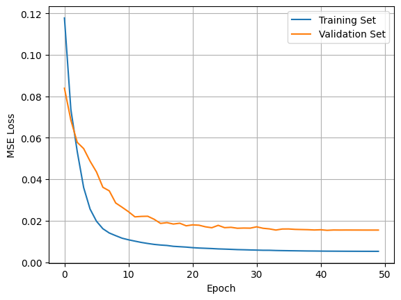
VIVformer training and validation loss trained on expreimental VIV data.

The training results show that the model is able to gradually decrease the MSE loss between targets and predictions. The loss on both the training set and the validation set seems to be decreasing and converging. We note that the VIVformer architecture used was heuristically optimized using a trial and error approach yielding 4 attention-residual layers, with 3 attention heads of 32 hidden units and a mlp-dim of 128 hidden units. In order to visualize the predicted vibrations, the forecasting as well as target data from a random sample of 36 continuous time steps from the validation set are shown below.

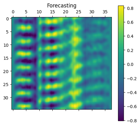
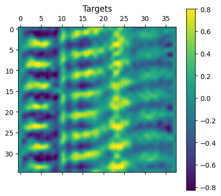
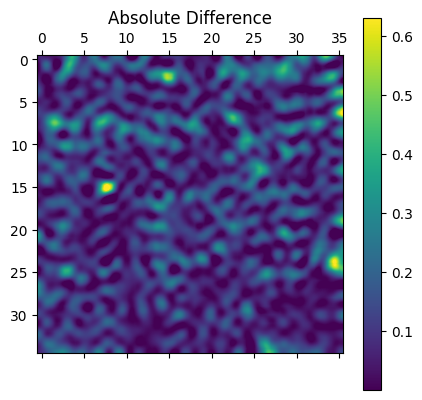
From left to right: Forecasting of the VIV on a ramndomly selected set of 36 continuous points from the validation set (for visualization of the predicted vibrations), target data from real experiments, absolute difference between targets and predictions.

As is evident from the visualized vibration predictions (above), the model can predict unseen experimental to reasonable accuracy. The expected modes are forecasted and the output is continuous. In addition, the absolute difference is almost everywhere small, although some inaccuracies do occur in the predictions. A meaningful question to ask would be how well does the model predict the root mean square (RMS) of the vibrations which gives us a sense of the prediction capabilities on average. Below we plot the RMS of the forecasted as well as the experimentally observed vibrations.

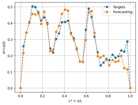
Root mean square (RMS) of the forecasted VIV as well as the experimentally observed. RMS displacement is shown on the y-axis while span (body position) is shown on the x-axis. Reasonably accurate agreement is evident between forecasting and experimental observations.

The RMS result shown above shows that the model can predict the vibrations reasonably accurately on average. This is a particulary important result as it allows for direct benchmarking of this method against semi-empirical models which can only predict the average vibrations.

Although this is not recommended practice as we described earlier, we attempt to make auto-regressive predictions using our model. That is, we start with 20 time steps of recorded vibrations as input and then use the model’s predictions gradually as more and more inputs. By 20 time steps, there would be no observed data input to the model; it would only be predicting on its outputs. The auto-regressive results are shown below.

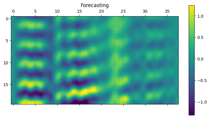
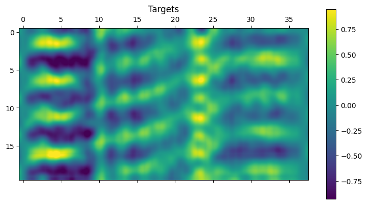
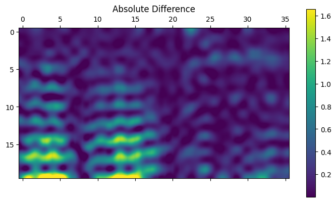
From left to right: Auto-regressive forecasting of the VIV on a randomly selected set of 20 continuous points from the validation set, target data from real experiments, absolute difference between targets and predictions. We show 20 time steps as we assess the models capability to predict as many time steps as it uses as input.

Albeit the mode shapes are consistent and remain physical looking, it appears that the magnitude of the response grows with time. As expected, errors accumulate and the forecasting becomes more and more innacurate as time evolves. This can also be clearly visualized in the absolute difference plot (on the very right) where the difference increases with time.

In conclusion, with respect to training on real data, the transformer is reasonably accurate in terms of forecasting future motions given a sample of the experimental data. The model trains well on the MSE loss and seems to converge in about 50 epochs. The wall time of training does not exceed a few minutes on a Google-Colab T4 GPU machine.

The hyper-Real (Gen-AI data) Deal

So far we have established that the VIVformer architecture can model the physical VIV of flexible bodies reasonably accurately. This section will mainly focus on addressing the question of whether synthetic VIV data generated using our VAE are physical: that is, whether the physical properties of the vibrations are preserved during the generative process. In order to address this question, we will train the VIVformer on synthetic data only and then test the trained model on the real data.

Sixty arrays of 36 time steps at 36 locations (this can be though of as generating 60 images similar to the ones shown in previous section “Vibration Data as Images”) were generated using the VAE trained on real experimental data. The synthetic VIV data were then organized in input and target sequences by creating a dataset and dataloader to train the VIVformer. Training was done exactly as described in section “The Real (data) Deal” with the only difference being the training data; in this case training data were only synthetic. The same split of 80% for training/validation was used on the synthetic data. The training results were as follows.

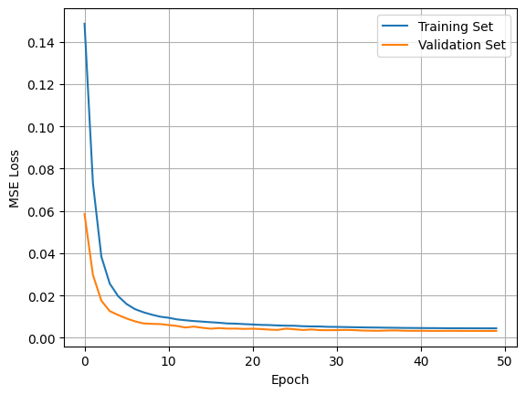
VIVformer training and validation loss trained on synthetic VIV data.

The VIVformer architecture seems to train on the sythetic data well. We note that both the training and validation data are from the synthetic dataset and as such we expect that they should be very similar data. We train for 50 epochs and the results seem to reach convergence. In this case we note that the error on the validation set (calculated during each epoch after optimizing on the VIVformer on the training set) seems to be be consistently smaller than the error on the training set (on average). We expect that eventually the training loss would become smaller than the validation loss although more training epochs would be required, perhaps leading to overfitting our model. Given the training results, we can be confident that the VIVformer has learned to predict the synthetic data well.

The more important question is however, whether the VIVformer trained on the synthetic data can accurately forecast the real experimental data. Below we show the predictions of the VIVformer on the real experimental data. We underscore that the VIVformer has NOT seen a single real datum during training: the model has trained on synthetic data only!

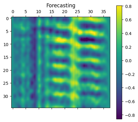
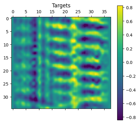
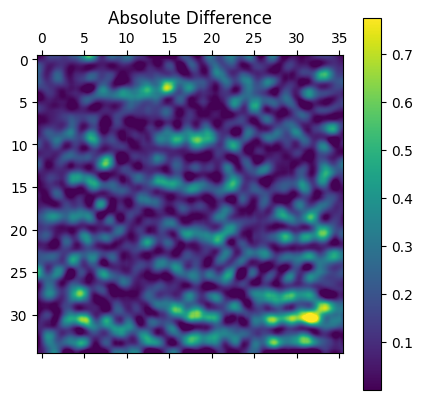
From left to right: Forecasting real VIV on a ramndomly selected set of 36 continuous points from the experiments, target data from experiments, absolute difference between targets and predictions. We note that the model has trained on synthetic data only and has never seen any real data!

Albeit the VIVformer has not seen any real data during training, it is surprisingly reasonably accurate in predicting real data! Although certainly not perfect, the predictions are sensible. The root-mean-square of the vibrations forecasted and observed are shown below.

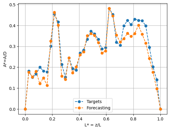
Root mean square (RMS) of the forecasted VIV plotted on top of the RMS of the experimentally observed VIV. RMS displacement is shown on the y-axis while span (body position) is shown on the x-axis. Reasonably accurate agreement is evident between forecasting (after training on synthetic data only) and experimental observation.

As is evident in the above figure, the VIVformer can make reasonably accurate predictions of the RMS of the vibrations. Both the trends and amplitudes are reasonably accurately estimated.

Since the VIVformer has never trained on real data but can reasonably accurately predict them, we conclude that at least part of the physicality of the real data is preserved during the genrative process of the VAE. In a sense, the VAE can be though of not just as a generator which makes realistic-looking data but as a tool which learns the underlying structure and mechanisms of the physical process which generates the data; it can thus be used to better understand the data and perhaps even the physical generative process. We conclude that our VAE could certainly be used to augment scarse datasets of VIV data and in addition, that it is a powerful tool that could potentially be used to study the underlying mechanisms of the physical generative process by studying the artificially generated data!

Conclusions

In this work, a data driven approach is employed to study physical system vibrations. Two main topics are explored: 1. Generative models for creating synthetic data similar to those obtained via physical processes and 2. employing transformers and the attention mechanism in order to model and forecast physical vibration data.

A variational autoencoder is trained on physical vortex-induced vibration data in order to generate sythetic data of the vibrations. The VAE is certainly able to generate data which resemble the physical data visually. Moreover, the generative process is confirmed to preserve the physicality of the data at least partially: a transformer trained on synthetic data only is capable of predicting real experimental data to reasonable accuracy. In that sense, the VAE can be viewed as a tool which learns the underlying physical traits of the data and can be used not only to augment physical datasets but also to simulate and understand the underlying physical mechanisms by examining synthetic data. With that being said, a recommended future research direction would be to examine whether the outputs of the VAE satisfy physical equations of interest and how those could perhaps be included as an additional loss term when training the VAE, i.e. having a physics-informed decoder network.

A transformer architecture for forecasting unsteady and nonstationary vortex-induced vibrations, the VIVformer, is developed. The VIVformer architecture combines multi-head attention modules and fully conncted network modules with residual connections in order to model and forecast the physical vibration time-series in both space and time. The optimized VIVformer architecture can forecast flexible body VIV in time-space to reasonable accuracy both instantaneously and on average. Testing the performance of the VIVformer while gradually decreasing the input information would yield a deeper understanding in the capabilities of the architecture; in addition, testing the extended time horizon predictions of the model would cretainly be a recommendation for future research.