Recovering Latent Variables with VAEs despite Training Bias

Final Project Blog

Introduction

In this age of abundant unlabeled data, unsupervised learning is capitalizing to power the generative models that are eating the world. Large Language Models and Diffusion models are focalizing most of the mainstream hype and therefore siphoning attention from other generative models. In particular, the Variational Autoencoders (VAE) is a model architecture that has been arguably overlooked in the recent onslaught for scaling transformer and diffusion-based models. VAEs are a promising latent variable model that allows for the learning of disentangled latent variables that model data.

As models scale in size, so is concern for the lack of interpretability associated with Neural Networks. Latent variable models offer a solution to this problem since they can learn variables that factorize the data generation process. VAEs are particularly well suited for learning latent variables in an unsupervised setting since they use an unsupervised learning objective and are regularized to learn disentangled encodings of our data. VAEs have been applied in a broad breadth of settings, such as classifying out-of-distribution data , fair decision making , causal inference , representation learning, data augmentation, and others. Although VAEs have demonstrated the capability to recover ground truth latent variables, they often recover mock factors that can generate the training dataset but differ mechanistically from the ground truth data generation process. For instance, in lecture we demonstrated that a VAE trained on cartoon images of rivers learned to encode aggregate river curvature as a latent variable. The ground-truth data-generating random variables were an ordered set of Bernoulli random variables indicating if the river angeled its trajectory to the left or to the right at the particular timestep. The VAE’s shortcoming in recovering the real latent variables is expected from a Bayesian perspective, since we assume an isotropic Gaussian prior for continuous latent variables, and impose a bottleneck on the number of latent variables. Even though we do not recover the ground-truth data generating random variables, we learn latent variables that are qualitatively useful and capture macro latent phenomenons about the data. This segways into an interesting question—when do VAEs fail to recover useful latent variables?

In particular, we will choose the setting in which our training data is biased, but we still seek to learn insightful representations of the data. This is an especially well-motivated setting, since in unsupervised learning, we often do not have any guarantees about the distribution of our training data, yet we still aim to learn generalizable latent variables. It would be ideal if VAE’s ability to recover generalizable latent variables is robust to training bias. Relating to the cartoon example from lecture, if the probability parameter for the data-generating random variables was skewed so that right-curving rivers are more likely (i.e. $P(\text{right}) = 0.9$ instead of $P(\text{right}) = 0.5$), would we still learn useful latent variables, or would latent variables instead model what we assume to be observational noise? If we learn the former, then we would still be able to sample in latent space to generate left-curving rivers. Intuitively, we will not be able to generate samples out of distribution with the training data (i.e. left curving rivers), however this may not be the case due to the way VAEs assume a prior. In this project, we will examine this setting to determine if higher regularization of the prior increases model robustness to training bias.

Background

VAEs are useful as encoders for downstream tasks, and as generative models. Compared to vanilla autoencoders, they offer significant advantages, since they provide some assurances regarding the distribution of its latent variables. Unlike VAEs, standard Autoencoders can have arbitrarily distributed embeddings, making them poor generative models, since there is no straightforward way to sample in latent space so that we generate samples in distribution with our training data. VAEs are similar to standard Autoencoders, however, they are trained with a modified loss function that ensures the learned embedding space is regularized towards an isotropic Gaussian (there exist alternative choices regarding which distribution we regularize towards, but Gaussian Mixture Models are the most popular as it stands due to their simple parameterization and empirical success). Additionally, instead of simply compressing the input with a neural network during the forward pass, the encoder of a VAE outputs a mean and covariance, defining a distribution from which we sample to obtain our latent variables.

Since the VAE loss function regularizes our latent variables towards an isotropic Gaussian, encoded data is both disentangled and interpretable. To use trained VAEs as generative models, we simply sample latent variables i.i.d. from the Gaussian distribution and pass it through the VAE decoder to generate samples in distribution with our training data. VAEs also offer significant advantages as encoders, since regularization encourages them to learn factored, disentangled representations of the data. Finally, VAEs are particularly well-suited for interpretability since regularization encourages each latent variable to capture a unique aspect of the data.

There has been significant prior work studying regularization and choice of priors in VAEs. Notably, $\beta$-VAE introduces the beta parameter to control the degree to which the VAE loss function penalizes the KL divergence of the latent variable distribution with the chosen prior (an isotropic Gaussian in their case). Higgins et al. demonstrate that introducing the beta parameter allows the VAE encoder to learn quantitatively more disentangled latent variables. They introduce a novel quantitative metric to evaluate the disentanglement of latent space and show that $\beta$-VAE improves on existing methods. Furthermore, they train a $\beta$-VAE on a dataset of faces (celebA) and qualitatively show that $\beta$ regularization allows for the factorization of previously entangled latent variables such as azimuth and emotion.

There have been several iterations on $\beta$-VAE such as Factor-VAE . Kim and Mnih point out that although $\beta$ regularization improves disentanglement in embedding space, it does so at the cost of reconstruction quality. To reduce this trade-off and still encourage disentanglement, they introduce a term to the VAE loss function that penalizes the KL divergence between the joint distribution and the product of the marginals, instead of with an isotropic Gaussian as in $\beta$-VAE.

Selecting an appropriate data prior is fundamental when performing Bayesian inference. In vanilla VAEs, we often assume an isotropic Gaussian prior for our latent variables, however, this is not always a good assumption, making it difficult to converge . Miao et al. propose InteL-VAE, a VAE architecture capable of learning more flexible latent variables that can satisfy properties such as sparsity even when the data has significant distributional differences from a Gaussian. Their contributions allow for higher customizability of latent variables while bypassing many of the convergence issues commonplace with other methods that assume non-Gaussian priors.

Since that under ideal conditions, VAEs recover factorized latent variables, causal inference has become a standard setting for their application. Madras et al. propose structured causal models to recover hidden “causal effects” with the aim of improving fairness when presented with biased data . They specify a framework where we want to recover the latent factors so that decision making in applications such as loan assignment and school admissions can be approached fairly. Admiddetly, Structured Causal Modeling (CSM) is arguably a better setting for futher work on our proposed research question. However, this field is largely outside of the scope of the course, so we will only observe that Madras et al. utilyze a model where causal factors, which are analaguous to our ground truth latent variables, affect a decision and an outcome, and that they utilyze a Bayesian framework to perform variational inference. Future iterations of our research should borrow methods from this field of Mathematics for maximum impact. Louizos et al. propose the Causal Effect VAE , marrying the adjacent fields and setting the stage for future research.

Although there is plenty of research adjacent to our particular question of interest, $\beta$-VAE investigates how $\beta$-regularization affects disentanglement, but not robustness to training bias. Other works that investigate the ability of latent variable models to recover the ground truth in the presence of training bias are not concerned with $\beta$-regularization. $\beta$-regularization has been shown to be effective, in addition to being extremely simple to implement, compared to other regularization techniques. Thus it is an ideal candidate for directed research on how regularization affects VAE robustness to training bias. Our question is novel, supported by adjacent research, and reasonable to implement with the resources available to an undergraduate student.

Set-up and Methods

Data

More concretely, suppose that there exists a data generating function $\mathcal{G}: Z \to X$ that generates our training dataset given random variables $Z \sim p_{\text{data}}$. For simplicity, our data will be nxn grids of squares, where the intensity of each square is deterministically proportional to its respective random variable. To create our training dataset, we sample $n^2$ random variables from an isotropic Gaussian distribution with mean $\mu$ and covariance I. We then apply a sigmoid activation to the random variables so that values are in the range [0,1]. We then create a mn x mn image with mxm pixel grids for each random variable. Finally, we add Gaussian noise to the image. We choose n=3, m=7, and train a VAE for each value of $\mu$ in the set {0, 1/2, 1, 3/2, … 5}.

Training Data

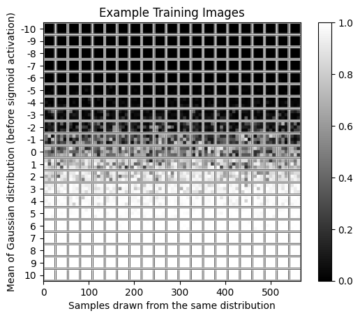
The following figure shows example training images before noising. Each row has 21 images drawn from the distribution defined by applying a sigmoid activation to a normally-distributed random variable with variance 1 and mean specified by the row index.

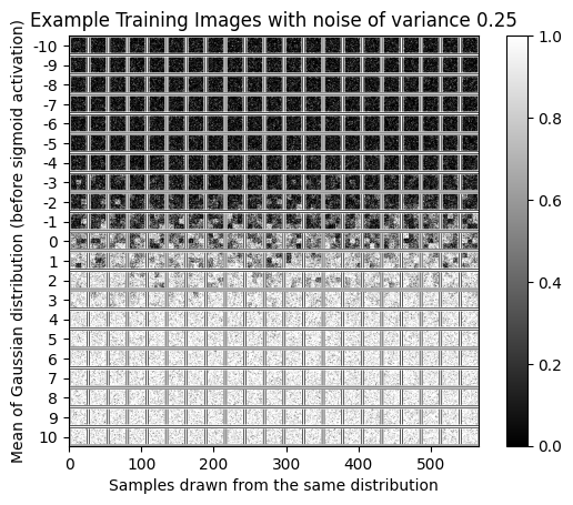
And here are some images with some noise added.

Test Dataset

To create our test dataset, we discretize the domain of latent variables by binning. We then enumerate all possible combinaation of latent variables, and generate corresponding images without adding noise. We restict the domain generating variables to {0.1, 0,5, 0.9}, and enumerate all possible combination. This yields a test dataset of 19683 images.

Example Test Images

Training

With this setup, the structure of our latent space matches that of the ground-truth latent variables, creating an appropriate setting in which to test how training bias and regularization affect the quality of learned models. Our pipeline is as follows. We train a VAE on its associated training set by maximizing the ELBO. After T training steps, we then train a linear projection head from the ground-truth latent variables to our learned latent variables. Even if we fully recover the ground-truth latent variables in our model, there is no assurance that we will not learn some permutation of the ground-truth latent variables. Thus in order to test if a particular latent variable was learned in our model, we must utilize such a projection to map from ground truth to learned latent variables, then decode the sample and evaluate the generated image.

Although the Mutual Information between the ground truth latent variables $z \sim p_z$ and the learned latent variables $\hat{z} \sim p_\hat{z}$ would be a more encompassing gauge if the VAE recovered the latent variables, using a linear projection in lieu of a Mutual Information estimator such as MINE is justified for the following reasons. Namely, we assume an isotropic Gaussian during training, so a good VAE will learn disentangled latent variables that will be off by at most a rotation from the ground truth latent variables. Furthermore, we control the data generation process so that data is generated by $n^2$ normally distributed random variables. Thus we can assume that a linear projection is sufficient to recover the ground truth latent variables from our learned latent variables. Furthermore, given the time constraints and resources allocated for this project, simply training a linear projection and taking the final mean squared error as a proxy for mutual information allows for simpler implementation.

We train with the Adam optimizer.

Hyperparameter	Value
VAE training steps	10000
Linear Projection Training Epochs	3
Training noise mean	0
Training noise variance	0.25

Results

Training Observations

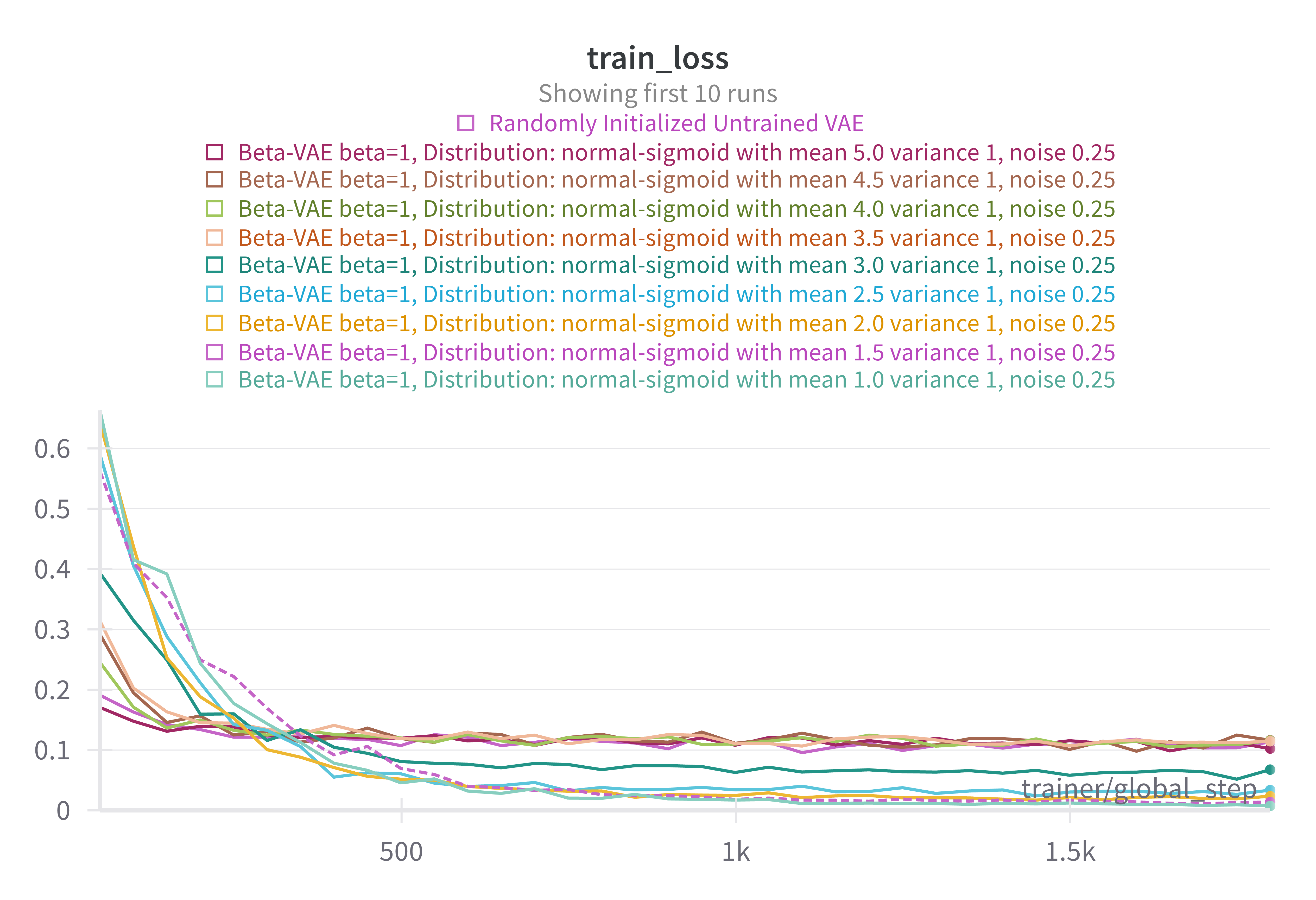
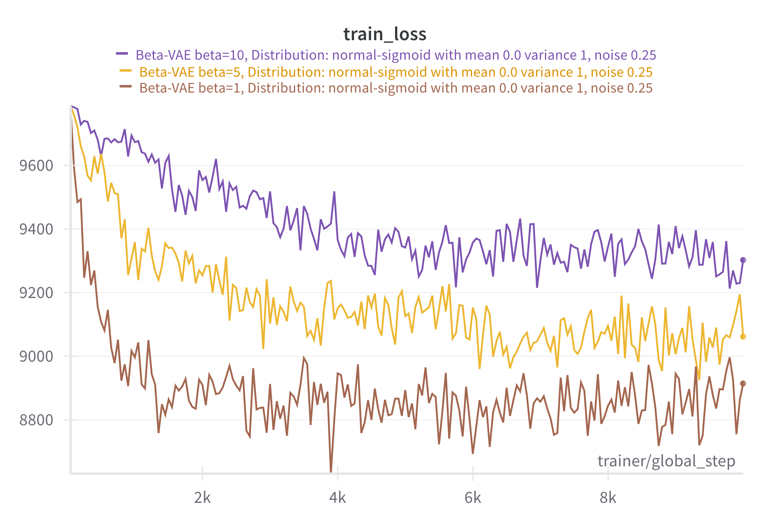
During the unsupervised training phase where we train the various VAE models on their respective training sets, we observe that dataset choice and penalization of the KL divergence (beta hyperparameter) have consistent effects on the training curves. The following charts demonstrate that increased penalization of the KL divergence results in higher training loss, as well as nosier training loss and longer convergence times. This is expected since higher regularization directly increases the loss and its associated noise. We approximate the KL divergence by drawing one sample, which is highly variable, but tends to work emperically. We also observe that higher training bias (i.e. higher pre-activation mean of the pre-activation data generating latent variables) results in higher training loss. As we increase this training bias, it becomes harder and harder to disambiguate latent features from noise. Thus models learn uninterpretable latent variables and poor decoders that learn to trivially output the dominating color (white).

Training Curves Varying Training Distribution

Training Curves Varying $\beta$-Regularization

Evaluation

The following figure shows a heat map of our Proxy for measuring Mutual Information (which we will refer to as PMI) between the learned latent variables $\hat{Z}$ and the true latent variables $Z$.

Note that when we randomly initialized a VAE and then trained linear projections from the ground truth latents to recovered latents, we achieved an PMI 0.1121 (averaged over 3 runs with identical training parameters). The heatmap shows that we almost completely recovered the ground-truth latent variables with low regularization and low training bias. As training bias increases, the model recovers less and less informative representations of the true latent variables.

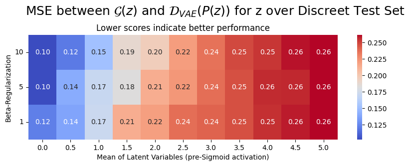
Another heuristic that we can utilize to estimate the Mutual Information between the recovered latents and the ground truth latents is the mean squared error between $\mathcal{G}(z)$ and $\mathcal{D}_\text{VAE}(P(z))$ averaged over our test set, where P is the learned linear projection from $Z \to \hat{Z}$ and $\mathcal{D}_\text{VAE}$ is the VAE decoder. The following figure heatmap visualizes this figure.

Conclusion and Future Work

From the collected data, it is visually clear that there exists a relationship between $\beta$-regularization and training bias. In both heat maps, there are reasonably well-defined diagonal level surfaces, indicating that there is some relationship between regularisation towards an isotropic Gaussian prior and robustness to training bias. Validation and further experiments are required to legitimize this conclusion, however, these experiments are an indication that conscious regularization can be a useful technique to mitigate training biases of a particular form. At this point, further work is required to interpret the results, since it is not clear why we seem to observe inverse relationships between the $\beta$-regularization and training bias when we involve the decoder.

It is also worth noting that during pretraining, VAEs were trained for a fixed number of training steps, and not until convergence. Thus it is highly plausible that models with higher $\beta$-regularization (i.e. models with $\beta > 1$) were not trained to completion, and therefore can not be fairly evaluated with mutual information estimators without further training. Given my computational and temporal constraints, it was not reasonable to run experiments with longer training. Future work will have to validate my findings by pretraining for longer and testing a finer resolution of $\beta$ parameters. Finally, it will be interesting to expand this work to more interesting datasets such as celebA and inject training bias by resampling the dataset according to some variables such as hair color or skin tone. Once we move beyond the assumptions assured by pet data, we can reevaluate what relationships hold true as we gradually add the complexity inherent to the real world.